|
FEATool Multiphysics
v1.16.5
Finite Element Analysis Toolbox
|
|
FEATool Multiphysics
v1.16.5
Finite Element Analysis Toolbox
|
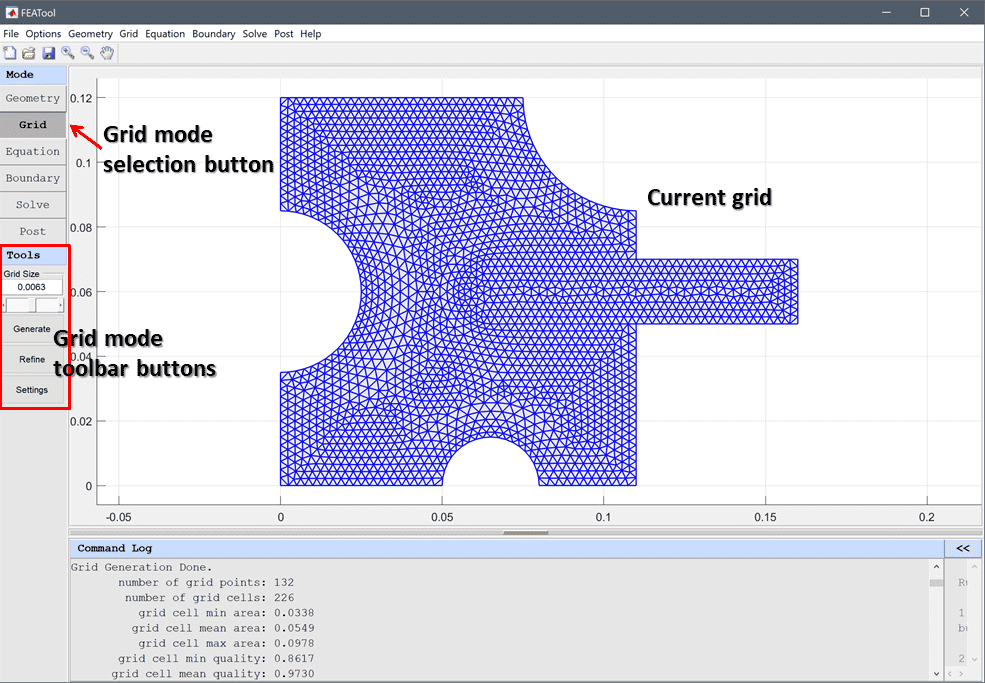
After a model geometry has been defined, a computational grid or mesh must be generated to allow for the finite element discretization. This section describes how to create or import a compatible grid.
Grid mode can be selected by pressing the ![]() mode button or corresponding menu option. In grid mode the toolbar buttons allow for grid generation, refinement, and accessing the advanced grid generation settings.
mode button or corresponding menu option. In grid mode the toolbar buttons allow for grid generation, refinement, and accessing the advanced grid generation settings.
The Grid Generation Settings dialog box shown below
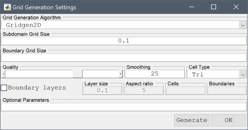
allows for selecting the mesh and Grid Generation Algorithm
The built-in default algorithm should work well in most cases and the other algorithms are optional. Specifically the Robust algorithm is appropriate for difficult to mesh 3D geometries and faceted geometries (such as from STL and OBJ CAD formats).
The Subdomain Grid Size and Boundary Grid Size edit fields can be used to prescribe maximum grid sizes for subdomains and boundaries. Accepts a scalar or space separated list of real numbers (one entry for each subdomain or boundary).
The following options are only available and enabled by a subset of grid generation algorithms.
The Quality slider allows setting the target mesh quality. For the Robust algorithm this will correspond to the detail level included features (high quality will include more and finer features of the input geometry).
The number of grid Smoothing steps can be specified in the corresponding edit field.
Cell Type shows which mesh cell types are available Tri, Quad, or Tet. Quadrilateral mesh generation is available with the Built-in and Gmsh algorithms in 2D.
The Reparametrization Angle is available with the Robust and Gmsh mesh generators for STL faceted geometries to set prescribe a feature angle for boundary segmentation (post mesh generation). See the corresponding section below for more details and manual boundary assignment. This parameter is specified in degrees, with zero (0) disabling automatic boundary reparametrization.
Selecting the Boundary Layers checkbox enables mesh generation of structured boundary layers on boundaries (available in 2D with the Gridgen2D and Gmsh mesh generators). The height of the boundary layer can be specified with the Layer Size and also Aspect Ratio between cells. With Gmsh it is also possible to specify the number of mesh Cells in the boundary layer, and the boundary numbers to apply boundary layer generation to (Gridgen2D is limited to boundary layers around internal regions/holes).
Lastly, the Optional Parameters field allows for an additional string of space separated property/value pairs to be supplied to the grid generation call (which effectively appends the user defined options to the gridgen function call, for example 'waitbar' false would suppress the progress bar during grid generation). For the Robust mesh generation algorithm it can be used to pass on CSG operations on geometry objects (with for example 'formula' 'OBJ1 - OBJ2'). See the gridgen command for valid optional arguments that can be passed on.
The Grid menu also features some options to view, edit, and modify grid data. The Convert Grid Cells menu option is used to convert between triangular and quadrilateral cells in 2D, or between tetrahedral and hexahedral cells in 3D. View Subdomains... and View Boundaries... can be used to show resulting geometric entities and their corresponding numbering. This is the numbering used to assign different mesh sizes to different subdomains and boundaries for the built-in grid generator.
The View Selected Cells... menu option allows for specifying an expression to select and show a subset of grid cells, such as x>0 or x>0 & z<=0.5 (useful for viewing the interior of 3D meshes). In 3D, the option Boundary Numbering... is also available to view and modify the boundary numbering of the mesh, and which cells should be assigned to which boundaries. Lastly, the Grid Statistics... option shows mesh statistics such as grid cell quality for the current grid.
The Grid menu also supports the following import and export of grids through external files and to/from the main MATLAB workspace
3D faceted geometries, such as those from imported STL and OBJ CAD file formats, typically do not include enough information to clearly identify geometry boundaries. In such cases it is possible to manually perform boundary assignment of grid cells. Selecting the Boundary Numbering... Grid menu option opens the corresponding dialog box below.

The "Recaculate" button will try to automatically re-number boundaries with the chosen sharp Feature angle (effectively calling the gridbdr function).
The "Manual Boundary Editing/Selection" section allows for manually specifying and changing the boundary numbering. The edit field allows for a selection syntax for the forms x>0 and x>0 & z<=0.5 to select with the coordinates x, y, and z, and selection via boundary numbers as ib==1 or ib>=3 (where ib is the current boundary number) View Menu Options show and highlight the boundaries and cells corresponding to the selection expression. The Edit Selection button allows for manually reassigning a boundary number to the selection, and Delete Selection completely removes the selected cells from the list of boundaries.
FEATool Multiphysics also comes with optional and built-in support for the external mesh generators Gmsh and Triangle. External grid generators allow for different grid generation algorithms, control options, and meshing results, which can be useful if the built-in ones have a difficult time meshing a geometry. The Grid Generation Algorithm can be selected with the corresponding option in the Grid Generation Settings dialog box.
In addition to the external grid generator interfaces, FEATool also fully supports mesh import and export from the Dolfin/FEniCS (XML), GiD, and ParaView (VTK/VTP) formats.
If Gmsh or Triangle is selected as grid generation algorithm and FEATool cannot find the corresponding binaries, they will automatically be downloaded, and installed when an internet connection is available. Alternatively, the mesh generator binaries can downloaded from the external grid generators repository and/or compiled manually and added to any of the directories available on the MATLAB paths so they can be located by the FEATool program (external binaries are typically placed in the bin folder of the FEATool installation directory). (The grid generator binaries are expected to have the file extensions exe, lnx, mac for Windows, Linux, and MacOS platforms respectively.)
Should Gmsh installation fail, please manually download and install Gmsh from the original source reference (Gmsh version 4.6.0 is recommended as is has been tested and validated for use with FEATool).
FEATool allows importing and exporting finite element grids between FEniCS, GiD, Gmsh, OpenFOAM, ParaView (VTK), and Triangle formats with the corresponding impexp_dolfin, impexp_gid, impexp_gmsh, impexp_foam, impexp_vtk, and impexp_triangle functions. These functions can also be accessed from the Grid and Postprocessing menus of the FEATool GUI.
Gmsh msh files can be imported either into the GUI using the corresponding menu option, or the impexp_gmsh MATLAB function.
FEATool currently only supports Gmsh mesh file format version 2 (default in Gmsh versions 2-3), which was replaced with an incompatible format in Gmsh version 4.0 and later. When using FEATool to mesh geometries this is handled automatically.
However, one must take care when using Gmsh manually and ensure that Gmsh v4 saves and exports meshes in version 2 format. One can either start Gmsh with the command line argument -format msh2, for example
gmsh.exe -format msh2
or set the following option in the general or mesh specific Gmsh .opt file
Mesh.MshFileVersion = 2;
The option files can be generated by selecting Save Model Options or Save Options As Default in the File menu.
If there are issues importing the mesh into FEATool one can also optionally try to add the -save_all command line argument which corresponds to the Mesh.SaveAll = 1; .opt file option.
Due to the simple grid format syntax it is possible to manually import grids from other software. The process essentially consists of first exporting the grid point coordinates and grid cell connectivity data from the external grid generation tool into separate text files. Then import them into MATLAB, after which they can be reshaped and used by FEATool. The following steps describe the process
 load p.txt
 load c.txt
 n_sdim = size(p,1);
 a = gridadj( c, n_sdim );
 n_c = size(c,2);
 s = ones( 1, n_c );
b = gridbdr( p, c, a );
Alternatively, one can manually construct and set the boundary numbering, for example as
 [ix_edge_face,ix_cells] = find( a==0 );
 b = [ix_cells'; ix_edge_face'; ones(1,length(ix_cells))];
 b = [b; gridnormals(p,c,b)];
this creates a boundary array b where all external boundaries are joined. With additional boundary information one can now split the boundary edges and faces (columns) by assigning different boundary numbers (third row in b). A helpful function to use here is findbdr which allows one to find boundary numbers and column indices in to b by prescribing logical expressions such as x>0.5. For example
 [~,ix] = findbdr( struct('p',p,'c',c,'b',b), 'x>0.5', false );
 b(3,ix) = 2;
sets boundary number 2 on all boundary edges/faces where x>0.5 is true.
grid.p = p;
grid.c = c;
grid.a = a;
grid.s = s;
grid.b = b;
Optionally, one can also add the grid to an existing finite element GUI model by using the Grid Menu option
Grid > Import Grid > From MATLAB Workspace...
Select the created grid variable to import and press Import. This loads it into the local FEATool memory workspace of the GUI (note that this overwrites the existing fea grid data). Press the Grid mode button to update and show the new grid.
This section describes the format of the grid data structure that FEATool employs as well as advanced command line (CLI) usage such as manually creating and importing grids.
The grid format used by FEATool is specified in the grid struct with the following fields
| Field | Description | Size |
|---|---|---|
| p | Grid point coordinates | (n_sdim, n_points) |
| c | Grid cell connectivity | (n_vertices_per_cell, n_cells) |
| a | Grid cell adjacency | (n_edges/faces_per_cell, n_cells) |
| b | Boundary information | (3+n_sdim, n_boundary_edges/faces) |
| s | Grid cell subdomain list | (1, n_cells) |
The coordinates of the grid points are specified by an array p, with the row number indicating the i-th coordinate direction, and column number the corresponding grid point number.
Cell connectivities are specified in the c array, where each column point to the grid points (in p) making up each cell. The row index gives the local vertex number and the column index the cell number. Moreover, the grid points are numbered counterclockwise in each cell.
Adjacency, meaning pointers to neighboring cells, are specified in the a array. Similar to c the row index gives the local edge in 2D or face number in 3D (starting with the corresponding grid point in c) and the column index points to the cell number. If the edge/face is on an external boundary the corresponding entry in a is 0.
Boundary information is specified in the b array. The cell, edge/face, and boundary numbers are prescribed in the first to third rows. The last n_sdim rows consists of the outward pointing unit normals corresponding to each boundary cell edge/face.
A list of subdomain numbers for each cell is given in the s vector.
The various grid cells available in FEATool are defined in this section.
In one dimension only the simple straight line segment grid cell is available. Grid Example 1 shows how this can be defined and used.
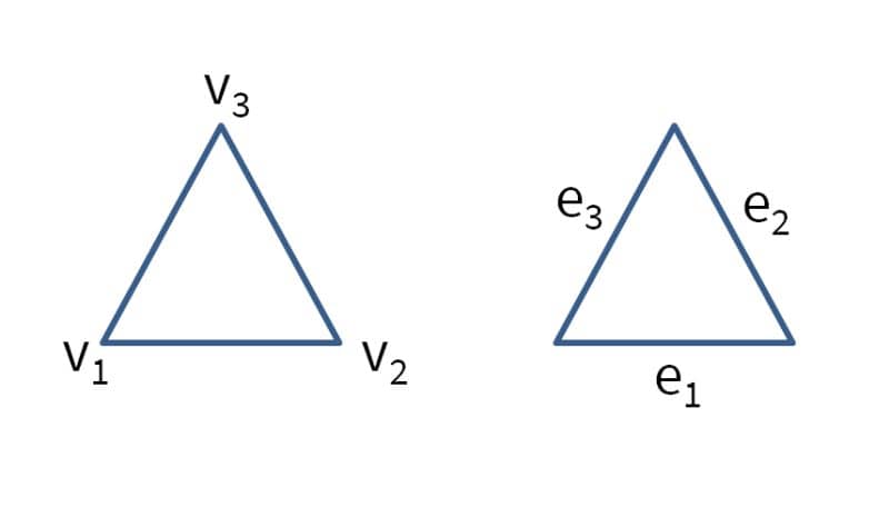
The 2D triangular grid cell is defined with vertices in counter clockwise order. Local edges ei are defined by the local vertices vi as
[ e1 ;    [ v1 v2 ;
  e2 ; =    v2 v3 ;
  e3 ]      v3 v1 ];
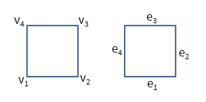
The quadrilateral grid cell is similarly defined with vertices in counter clockwise order. Local edges ei are defined by the local vertices vi as
[ e1 ;    [ v1 v2 ;
  e2 ;      v2 v3 ;
  e3 ] =    v3 v4 ;
  e4 ]      v4 v1 ];
The 3D tetrahedral grid cell is defined with vertices in counter clockwise order. Local edges ei are defined by the local vertices vi as
[ e1 ;    [ v1 v2 ;
  e2 ;      v2 v3 ;
  e3 ;      v3 v1 ;
  e4 ; =    v1 v4 ;
  e5 ;      v2 v4 ;
  e6 ]      v3 v4 ];
The local faces fi are defined by the local vertices vi as
[ f1 ;    [ v1 v2 v3 ;
  f2 ;      v1 v2 v4 ;
  f3 ; =    v2 v3 v4 ;
  f4 ]      v3 v1 v4 ];

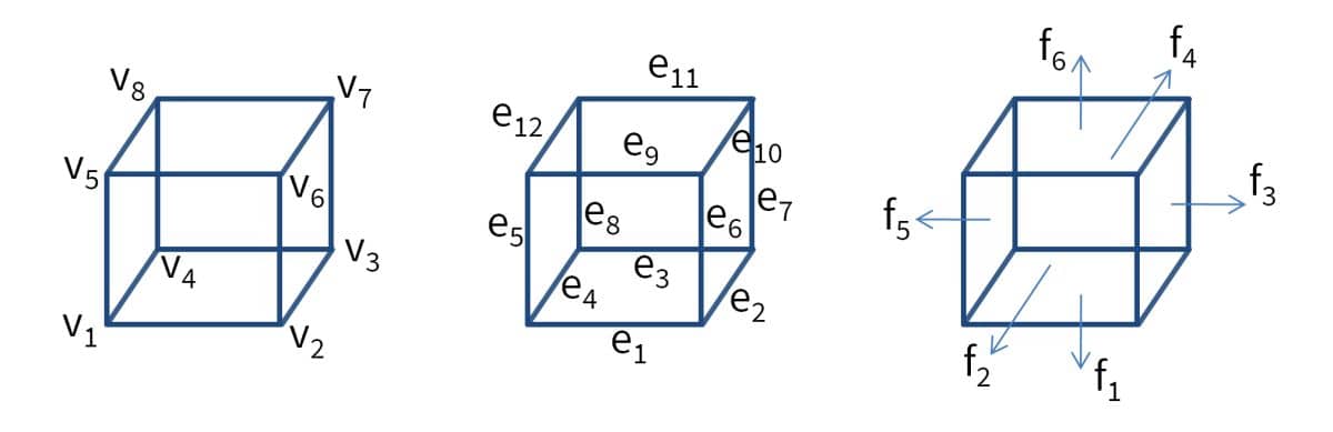
The hexahedral brick grid cell is defined with vertices in counter clockwise order. Local edges ei are defined by the local vertices vi as
[ e1  ;    [ v1 v2 ;
  e2  ;      v2 v3 ;
  e3  ;      v3 v4 ;
  e4  ;      v4 v1 ;
  e5  ;      v1 v5 ;
  e6  ;      v2 v6 ;
  e7  ; =    v3 v7 ;
  e8  ;      v4 v8 ;
  e9  ;      v5 v6 ;
  e10 ;      v6 v7 ;
  e11 ;      v7 v8 ;
  e12 ]      v8 v1 ];
The local faces fi are defined by the local vertices vi as
[ f1 ;    [ v1 v2 v3 v4 ;
  f2 ;      v1 v2 v6 v5 ;
  f3 ;      v2 v3 v7 v6 ;
  f4 ; =    v3 v4 v8 v7 ;
  f5 ;      v4 v1 v5 v8 ;
  f6 ]      v5 v6 v7 v8 ];
The following code can be used to manually define a one dimensional grid with 10 uniformly spaced cells on the line (0..1)
grid.p = 0:0.1:1;
grid.c = [1:10;2:11];
grid.a = [0:9;2:10 0];
grid.b = [1 10;1 2;1 2;-1 1];
grid.s = ones(1,10);
Alternatively one can use the grid utility function linegrid
grid = linegrid( 10, 0, 1 );
The plotgrid function can be used to plot and visualize a grid
plotgrid( grid )
A 2 by 2 unit square rectangular grid can be created with the following commands
grid.p = [repmat([0,0.5,1],1,3);0 0 0 0.5 0.5 0.5 1 1 1];
grid.c = [1 2 5 4;2 3 6 5;4 5 8 7;5 6 9 8]';
grid.a = [0 2 3 0;0 0 4 1;1 4 0 0;2 0 0 3];
grid.b = [1 2 2 4 4 3 3 1;1 1 2 2 3 3 4 4;1 1 2 2 3 3 4 4; ...
          0 0 1 1 0 0 -1 -1;-1 -1 0 0 1 1 0 0];
grid.s = ones(1,4);
The rectgrid function can also be used to create rectangular grids, in this case
grid = rectgrid( 2, 2, [0 1;0 1] );
As before the grid can be plotted, visualizing both grid point and cell numbers, with
plotgrid( grid, 'nodelabels', 'on', 'cellabels', 'on' )
Similarly, the boundaries can be visualized with the function plotbdr (subdomains can be visualized with plotsubd)
plotbdr( grid )
As FEATool also supports simplex triangular cells in two dimensions a grid consisting of quadrilaterals can easily be converted with the utility function quad2tri
grid = quad2tri( grid )
Reverse conversions can be made with tri2quad function which uses Catmull-Clark subdivision. In 3D the hex2tet and tet2hex functions perform similar conversions.
A more complex example, a grid for a rectangle with a circular hole can be created by first creating geometry objects (a rectangle and a circle), applying a formula to construct the geometry shape, and then calling the automatic unstructured grid generation function gridgen
% Geometry definition.
xmin  = 0;
xmax  = 1;
ymin  = 0;
ymax  = 1;
tag1  = 'R1';
gobj1 =  gobj_rectangle( xmin, xmax, ymin, ymax, tag1 );

xc    = (xmax-xmin)/2;
yc    = (ymax-ymin)/2;
r     = 0.25;
tag2  = 'C1';
gobj2 =  gobj_circle( [xc yc], r, tag2 );

geom.objects = { gobj1 gobj2 };
formula = 'R1 - C1';
geom = geom_apply_formula( geom, formula );
fea.geom = geom;

% Grid generation.
hmax = 0.1;
fea.grid = gridgen( fea, 'hmax', hmax );
As before the grid can be plotted, visualizing both grid point and cell numbers, with
plotgrid( grid, 'nodelabels', 'on', 'cellabels', 'on' )
The computational finite element library in FEATool supports FEM shape functions for structured grids (quadrilaterals in 2D and hexahedra in 3D). Although more difficult to generate automatically, structured grids are often computationally superior, allowing for higher accuracy with a smaller number of cells.
In FEATool, structured tensor-product grids of basic geometric shapes can easily be generated on the command line with the following MATLAB m-script functions
| Function | Description |
|---|---|
| linegrid | Create a 1D line grid |
| circgrid | Create a 2D structured circular grid of quadrilateral cells |
| holegrid | Create a 2D rectangular grid with a circular hole |
| rectgrid | Create a 2D rectangular grid of quadrilateral cells |
| ringgrid | Create a 2D grid of a ring shaped domain |
| blockgrid | Create a 3D structured block grid |
| cylgrid | Create a 3D structured cylindrical grid |
| spheregrid | Create a 3D grid for a spherical domain |

Moreover, the grid utility functions selcells, delcells, gridextrude, gridmerge, gridrevolve, gridrotate, and gridscale can be used to manually modify, transform, and join grids to more complex structures.
The figure below shows three examples of more complex grids created by using these functions.
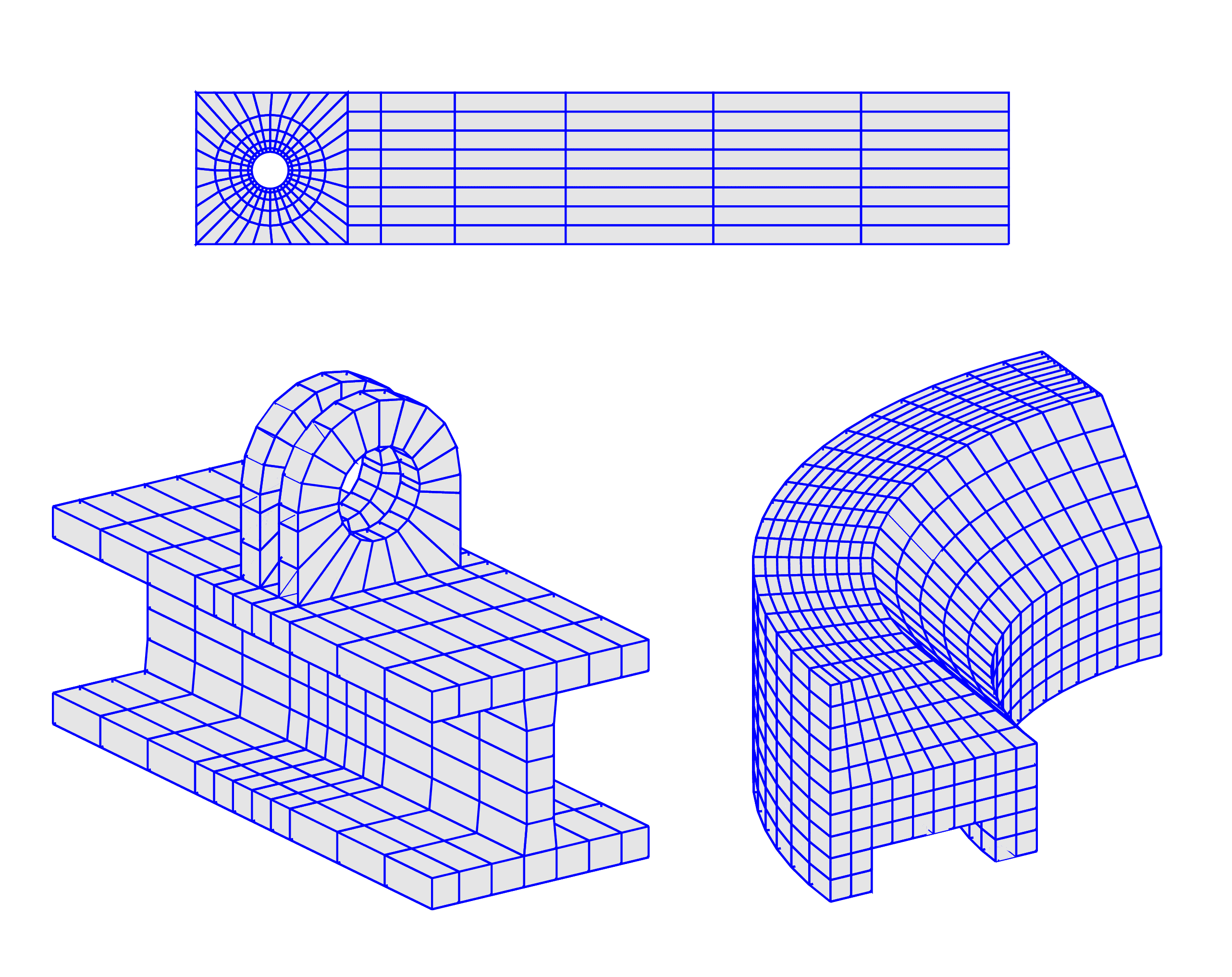
The first flow over cylinder benchmark grid is for example created with the following commands:
 grid1 = ringgrid( [0.05 0.06 0.08 0.11 0.15], ...
                   32, [], [], [0.2;0.2] );
 grid2 = holegrid( 8, 1, [0 0.41;0 0.41], 0.15, [0.2;0.2] );
 grid2 = gridmerge( grid1, 5:8, grid2, 1:4 );
 grid3 = rectgrid( [0.41 0.5 0.7 1 1.4 1.8 2.2], ...
                   8, [0.41 2.2;0 0.41] );
 grid  = gridmerge( grid3, 4, grid2, 6 );
And the lower right revolved grid with these commands:
 grid = rectgrid();
 grid = gridscale( grid, {'1-(y>0.5).*(y-0.5)' 1} );
 grid = delcells( selcells( ...
          '((x<=0.8).*(x>=0.2)).*(y<=0.2)', grid ), grid );
 grid = gridrevolve( grid, 20, 0, 1/4, 2, pi/2, 0 );
The last example with two brackets attached to an I-beam section is more complex:
 grid01 = ringgrid( 1, 20, 0.03, 0.06, [0;0] );
 indc01 = selcells( grid01, 'y<=sqrt(eps)' );
 grid01 = delcells( grid01, indc01 );

 grid02 = holegrid( 5, 1, .06*[-1 1;-1 1], .03, [0;0] );
 indc02 = selcells( grid02, 'y>=-sqrt(eps)' );
 grid02 = delcells( grid02, indc02 );
 grid2d = gridmerge( grid01, [5 6], grid02, [7 8] );

 grid1 = gridextrude( grid2d, 1, 0.02 );
 grid1 = gridrotate( grid1, pi/2, 1 );
 grid2 = grid1;
 grid1.p(2,:) = grid1.p(2,:) + 0.03;
 grid2.p(2,:) = grid2.p(2,:) - 0.01;

 x_coord = [ -0.08 linspace(-0.06,0.06,6) 0.08 ];
 y_coord = [ -0.2 -0.15 -0.1 -0.05 -0.03 -0.01 ...
              0.01  0.03  0.05  0.1  0.15  0.2 ];
 grid3 = blockgrid( x_coord, y_coord, 1, ...
                    [-0.08 0.08;-0.2 0.2;-0.08 -0.06] );
 grid4 = blockgrid( 1, y_coord, 5, ...
                    [-0.01 0.01;-0.2 0.2;-0.18 -0.08] );
 grid5 = grid3;
 grid5.p(3,:) = grid5.p(3,:) - 0.12;

 grid = gridmerge( grid1, 8, grid3, 6 );
 grid = gridmerge( grid2, 8, grid, 19 );
 grid = gridmerge( grid4, 6, grid, 24, 1 );
 grid = gridmerge( grid5, 6, grid, 33, 2 );
After, the grids have been created on the command line they can also be imported into the FEATool GUI (by using the Grid > Import Grid > From MATLAB Workspace... menu option).
Using quadrilateral grid cells are often advantageous to triangular cells in that they can provide somewhat more accuracy when aligned with geometry features and also tends to require less overall grid cells.
A mesh of quadrilateral grid cells can be created by using the gridgen function with quad as grid generation argument. This tries to align quadrilateral cell edges with immersed interfaces described by distance and level set functions. The algorithm then uses the zero level set contour from the distance functions to align grid cell edges with external geometry object boundaries. Furthermore, the cells are split in a way to treat edge cases such as when an interface segment crosses a cell diagonal. Optionally, the Built-in and Gmsh mesh generators also allows for quadrilateral mesh generation in 2D. Finally, it is also possible to subdivide triangles and convert into quadrilaterals, however the resulting grids are often of poor quality and not suitable for physics simulations.

The following functions are available for working with and processing grids
| Function | Description |
|---|---|
| gridgen | Unstructured automatic grid simplex generation |
| gridgen_scale | Grid generation with scaling of geometry objects |
| gridrefine | Refine a grid uniformly |
| gridstat | Show grid statistics |
| gridsmooth | Apply smoothing to a grid |
| gridextrude | Extrude a grid from 2D to 3D |
| gridrevolve | Extrude and revolve a 2D grid to 3D |
| gridrotate | Rotate a grid along a specified axis |
| gridscale | Apply scaling to a grid |
| gridmerge | Merge two grids along boundaries |
| gridnormals | Determine normal vectors to external cell edges/faces |
| get_boundary_layers | Find boundary layers |
| quad2tri | Convert a grid of quadrilateral cells to triangular cells |
| tri2quad | Convert a grid of triangular cells to quadrilateral cells |
| hex2tet | Convert a grid of hexahedral cells to tetrahedral cells |
| tet2hex | Convert a grid of tetrahedral cells to hexahedral cells |
| impexp_dolfin | Import and export FEniCS/Dolfin grid data |
| impexp_foam | Import and export OpenFOAM grid data |
| impexp_gid | Import and export GiD grid data |
| impexp_gmsh | Import Gmsh grid and postprocessing data |
| impexp_hdf5 | Import and export FEniCS/HDF5 grid data |
| export_su2 | Export grid data in SU2 format |
| impexp_triangle | Import and export 2D Triangle grid and polygon data |
| impexp_vtk | Import and export ParaView VTK grid data |
| gridcheck | Check grid for errors |
| gridadj | Create grid adjacency information |
| gridbdr | Create grid boundary information |
| gridbdre | Create 3D grid edge boundary information |
| gridbdrx | Reconstruct internal boundaries |
| gridvert | Create grid vertex information |
| gridedge | Create grid edge information |
| gridface | Create grid face information |
| findbdr | Find boundary indices and numbers |
| selcells | Find cell indices from an expression |
| delcells | Delete a selection of cells from a grid |
| plotbdr | Plot and visualize boundaries |
| plotsubd | Plot and visualize subdomains |
| plotgrid | Plot and visualize grid |