FEATool-Triangle Mesh Generator Integration
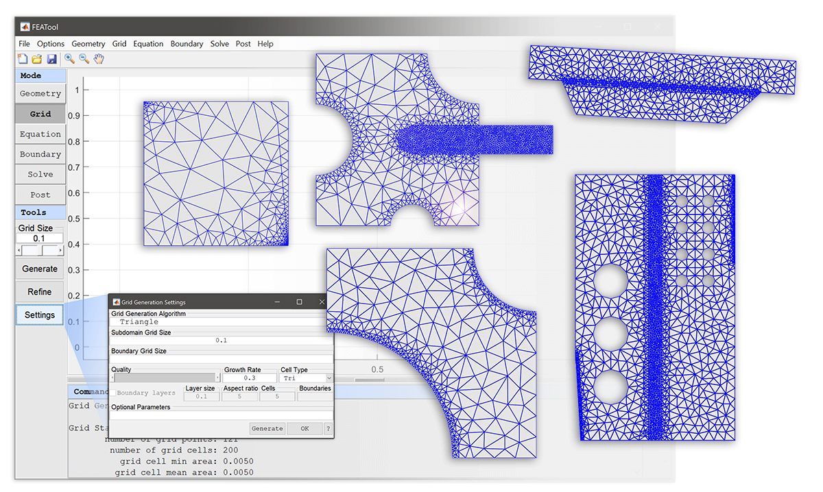
The fast and efficient 2D mesh and grid generator, Triangle, by J.R. Shewchuk’s is fully integrated with FEATool Multiphysics [1][2][3]. Both MATLAB command line interface (CLI) usage is supported with the gridgen function, as well as FEATool GUI usage by selecting the Triangle in the Grid Generation Settings dialog box.
Advantages of using Triangle compared to the built-in grid generation function is firstly the overall speed, as it is one of the fastest 2D unstructured mesh generators available (completely written in C code). Moreover, Triangle features better support for specifying the grid size in different subdomains and geometry regions, as well as on boundaries, allowing for greater flexibility and higher quality grids adapted to specific problems and geometries.
To evaluate the performance of Triangle and compare it to the built-in grid generator a simple benchmark test case was employed. The test case consisted of generating a uniform mesh for a unit circle with average grid sizes hmax = [0.1 0.05 0.025 0.0125 0.00625]. The normalized timings for using gridgen with the default algorithm
tic
geom.objects = { gobj_circle() };
grid = gridgen( geom, 'hmax', hmax );
t = toc
The time to mesh a unit circle in MATLAB and Octave with DistMesh, as well as with Triangle is shown in the figure below.
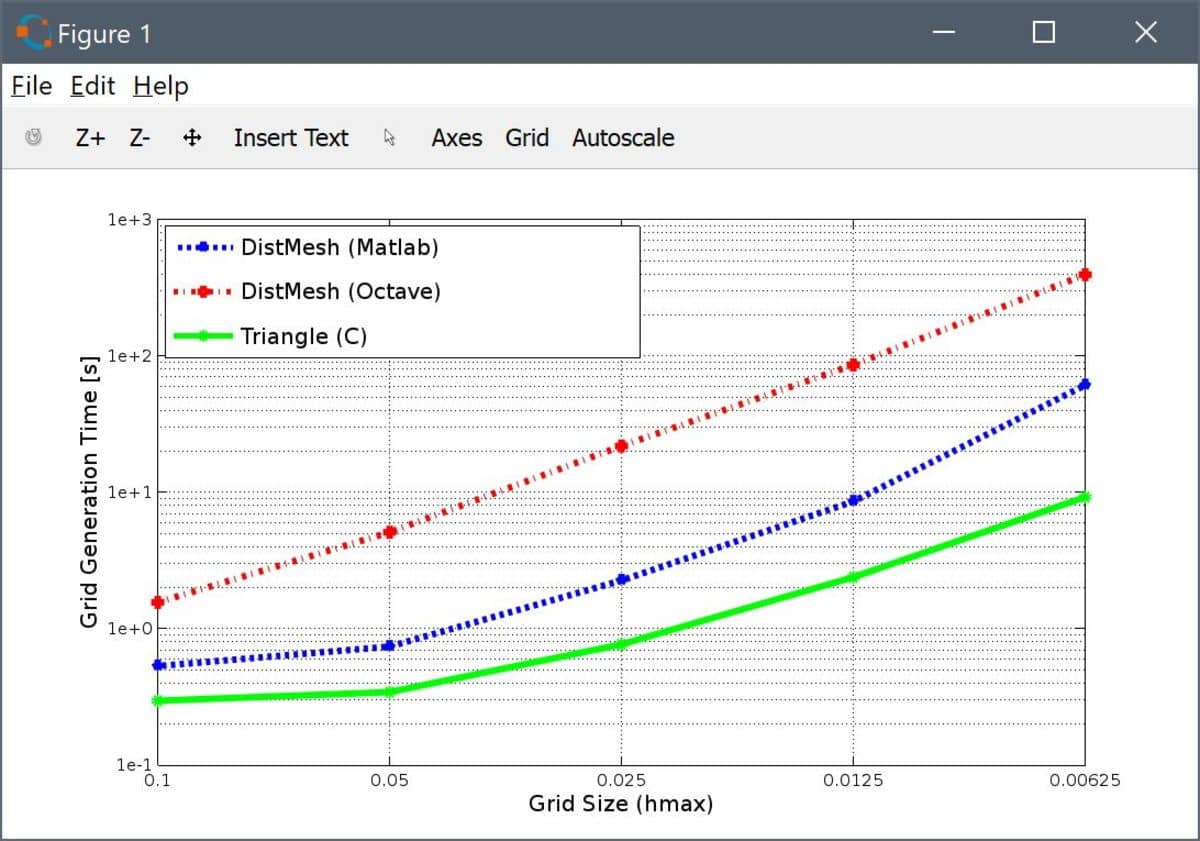
From the results one can see that for the finest grid (hmax = 0.00625, consisting of approximately 185000 triangles) required 10 seconds for Triangle, 1 minute for DistMesh and MATLAB, and close to 7 minutes for DistMesh and Octave (suffering from lack of Just-In-Time JIT compilation). Also note that the Triangle timings also includes time taken for IO export and import, that is the total time the user might typically see. Triangle can clearly offer magnitudes of speed improvements for basic two-dimensional unstructured grid generation.
Installation
First please ensure that the latest version of FEATool Multiphysics is installed. If Triangle is selected as grid generation algorithm but not found, FEATool will automatically try to download, (compile), and install the mesh generator binary into the userpath/.featool folder.
Should the Triangle installation or compilation fail, please manually download, compile, and install Triangle from the original source reference [1].
GUI Usage
Once installed, the Grid Generation Settings dialog box will feature a Triangle selection option from the Grid Generation Algorithm drop-down box. Moreover, the following options also apply to the Triangle mesh generation algorithm
The Subdomain Grid Size, hmax, indicates the target grid cell diameter, and can either be a single scalar prescribing the grid size for the entire geometry, or a space separated string of numbers (array) where the hmax values correspond to the generated subdomains.
Boundary Grid Size, hmaxb, is analogous to hmax but related to boundaries (edges). hmaxb can consist of a single scalar applicable to all boundaries, for example
0.1prescribing a mean cell edge length of 0.1 on every boundary. hmaxb can also be a numeric array with entries corresponding to individual boundaries, for example
[ 0.1 0.2 0.3 0.4 ]specifying cell edge length 0.1 for boundary 1, 0.2 for boundary 2 etc. Lastly, hmaxb can also be given as a cell array where each entry and boundary can be prescribed a single value for the mean cell edge size or a numeric array of grid point distributions (spanning 0 to 1) along the boundary. For example
{ 0.1 [0 0.1 0.5 1] 0.3 [1 0.8 0.2 0] }where here boundaries 1 and 3 are prescribed mean edge lengths 0.1 and 0.3, respectively. Boundary 2 is assigned nodes at parametrized positions 0, 0.1, 0.5, and 1 while boundary 4 the nodes are assigned in reverse.
The Quality slider (which corresponds to the_Triangle_ _q_ parameter, default 28 degrees) sets a minimum target angle (values less than 33 are generally acceptable, while higher values might prevent _Triangle_ convergence).
The Smoothing parameter specifies the number of post grid smoothing steps to perform (default 3).
The Generate grid button effectively calls the
gridgen function from the GUI with the
‘gridgen’ ‘triangle’ property/value pair as
input arguments, which in turn makes a system call to the Triangle
binary, after which the new grid is automatically imported and
displayed.
CLI Usage
On the MATLAB command line the gridgen function is used to call Triangle to generate an unstructured 2D triangular grid. The following syntax is used
grid = gridgen( SIN, VARARGIN, 'gridgen', 'triangle' )
where SIN is a valid FEATool fea problem struct or cell array of geometry objects. gridgen also accepts the following property/value pairs (VARARGIN).
Property    Value/{Default}            Description
-----------------------------------------------------------------------------------
hmax        scal/arr {0.1}             Target grid size for geometry/subdomains
hmaxb       scal/arr {[]}              Target grid size for boundary edges
q           scalar   {28}              Minimum target angle (quality)
nsm         scalar   {3}               Number of (post) grid smoothing steps
intb        logical  {false}           Keep internal boundaries
syscmd      string   {'default'}       Triangle system call command (default
                                       'triangle -I -q%f -j -e -a -A %s.poly')
compcmd     string   {'default'}       Triangle unix/linux compilation command
                                       ('cc -O triangle.c -lm -o triangle')
fname       string   {'fea_tri_UID'}   Triangle imp/exp file name (root)
fdir        string   {tempdir}         Directory to write help files
clean       boolean  {true}            Delete (clean) Triangle help files
instdir     string   {userpath/.featool}  Triangle installation directory
As also discussed above, among the properties hmax indicates target grid cell diameters, and is either a numeric scalar valid for the entire geometry or an array with hmax values corresponding to the subdomains. hmaxb is similar to hmax but a numeric array with a hmaxb values corresponding to the boundaries (including internal boundaries). q (default 28 degrees) specifies a minimum target grid size (values less than 33 are generally acceptable, while higher values might prevent convergence). nsm (default 0) the number of gridsmooth smoothing steps to perform. More detailed information regarding the mesh generation options can be found in the documentation for Triangle [1].
For more information about CLI usage access the function help by entering
>> help gridgen
### Grid Generation Examples
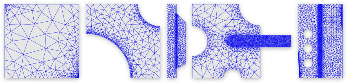
Unit square with uniform global grid size set to 0.1
 grid = gridgen( {gobj_rectangle()}, 'hmax', 0.1, 'gridgen', 'triangle' );
 plotgrid( grid )
Unit square with fine grid along the top boundary.
 grid = gridgen( {gobj_rectangle()}, 'hmax', 0.5, ...
                      'hmaxb', [0.5 0.5 0.01 0.5], 'gridgen', 'triangle' );
 plotgrid( grid )
Domain with fine grid along curved boundaries (number 5 and 6)
 geom.objects = {gobj_rectangle() gobj_circle([0 0],.6) gobj_circle([1 1],.3,'C2')};
 geom = geom_apply_formula( geom, 'R1-C1-C2' );
 grid = gridgen( geom, 'hmax', .1, 'hmaxb', [.1 .1 .1 .1 .01 .01], ...
                 'gridgen', 'triangle' );
 plotgrid( grid )
Two connected subdomains with refined grid along the shared boundary (9)
 geom.objects = { gobj_rectangle(-2e-3,0,-8e-3,8e-3), ...
                  gobj_polygon([0 -6e-3;2e-3 -5e-3;2e-3 4e-3;0 6e-3]) };
 hmax  = 5e-4;
 hmaxb = hmax*ones(1,9);
 hmaxb(9) = hmax/5;
 grid  = gridgen( geom, 'hmax', hmax, 'hmaxb', hmaxb, 'gridgen', 'triangle' );
 plotgrid( grid )
Component with fine grid on subdomains 2 and 3, and curved boundaries
 r1 = gobj_rectangle( 0, 0.11, 0, 0.12,  'R1' );
 c1 = gobj_circle( [ 0.065 0 ],   0.015, 'C1' );
 c2 = gobj_circle( [ 0.11 0.12 ], 0.035, 'C2' );
 c3 = gobj_circle( [ 0 0.06 ],    0.025, 'C3' );
 r2 = gobj_rectangle( 0.065, 0.16, 0.05, 0.07, 'R2' );
 c4 = gobj_circle( [ 0.065 0.06 ], 0.01, 'C4' );
 geom.objects = { r1 c1 c2 c3 r2 c4 };
 geom = geom_apply_formula( geom, 'R1-C1-C2-C3' );
 geom = geom_apply_formula( geom, 'R2+C4' );

 hmax  = [0.0015 0.02 0.0015];
 hmaxb = 0.02*ones(1,34);
 hmaxb([8:12]) = 0.0025;
 grid  = gridgen( geom, 'hmax', hmax, 'hmaxb', hmaxb, 'gridgen', 'triangle' );
 plotgrid( grid )
Complex geometry with several holes and subdomains
 w = 10e-4; L = 3*w; H = 5*w;
 p1  = gobj_polygon( [w/10 0;L 0;L H-H/3;L H;0 H;0 H/3], 'P1' );
 r1  = gobj_rectangle( (L-w/4)/2, (L+w/4)/2, -sqrt(eps), H, 'R1' );
 c1  = gobj_circle( [2*w/3 3*w], w/3, 'C1' );
 c2  = gobj_circle( [2*w/3 2*w], w/3, 'C2' );
 c3  = gobj_circle( [2*w/3 1*w], w/3, 'C3' );
 c4  = gobj_circle( [L-w/2 4.5*w], w/8, 'C4' );
 c5  = gobj_circle( [L-w   4.5*w], w/8, 'C5' );
 c6  = gobj_circle( [L-w/2 4*w], w/8, 'C6' );
 c7  = gobj_circle( [L-w   4*w], w/8, 'C7' );
 c8  = gobj_circle( [L-w/2 3.5*w], w/8, 'C8' );
 c9  = gobj_circle( [L-w   3.5*w], w/8, 'C9' );
 c10 = gobj_circle( [L-w/2 3*w], w/8, 'C10' );
 c11 = gobj_circle( [L-w   3*w], w/8, 'C11' );
 geom.objects = { p1 r1 c1 c2 c3 c4 c5 c6 c7 c8 c9 c10 c11 };
 geom = geom_apply_formula( geom, 'P1-C1-C2-C3-C4-C5-C6-C7-C8-C9-C10-C11' );

 hmaxb = w/5*ones(1,59);
 hmaxb([5 9]) = w/50;
 grid  = gridgen_triangle( geom, 'hmax', w./[5 20 5], 'hmaxb', hmaxb, 'gridgen', 'triangle' );
 plotgrid( grid )
Usage Notes
For geometries with multiple and overlapping geometry objects the actual subdomain numbering will generally not correspond to the geometry object numbering (two intersecting geometry objects will for example create three or more subdomains and several internal boundaries). In this case the actual subdomain and boundary numbering for vector valued hmax and hmaxb arrays can easiest be visualized and determined by first creating a coarse grid and switching to Equation/Subdomain and Boundary modes, respectively.
Furthermore, in contrast to the standard gridgen function, gridgen_triangle can identify and include internal boundaries (with the intb flag on). These internal boundaries can also be subject to boundary conditions, or alternatively should be assigned neutral/symmetry (homogeneous zero Neumann) boundary conditions if they are to be considered non-active boundaries (acting as if they were not present and ignored).
The temporary Triangle generated poly and tri data files can be found in the specified fdir directory (default given by the MATLAB tempdir function).
Lastly, even if a specific boundary node distribution has been prescribed through the cell array hmaxb parameter, Triangle may insert additional nodes if necessary in order to achieve and acceptable grid quality (depending on the prescribed q parameter).
References
[1] The Triangle Mesh Generator home page.
[2] J.R. Shewchuk, Triangle: Engineering a 2D Quality Mesh Generator and Delaunay Triangulator, in Applied Computational Geometry: Towards Geometric Engineering (Ming C. Lin and Dinesh Manocha, editors), volume 1148 of Lecture Notes in Computer Science, pages 203-222, Springer-Verlag, Berlin, May 1996. (From the First ACM Workshop on Applied Computational Geometry).
[3] J.R. Shewchuk, Delaunay Refinement Algorithms for Triangular Mesh Generation, Computational Geometry: Theory and Applications 22(1-3):21-74, May 2002.