When generating grids and meshes for fully three-dimensional structures with constant cross section in one or more directions, it is often advantageous to first create a two dimensional grid and extrude it to 3D, rather than generate a full 3D grid directly. By using the extrusion technique more control over the grid cell distribution can be achieved resulting in less dense and more computationally efficient grids.
The built-in gridextrude function supports extrusion of both quadrilateral to hexahedral and triangular to tetrahedral grid cells. Unstructured triangular to tetrahedral extrusions are carried out via a prismatic substep (each triangle is first extruded to a prism which is then split into three tetrahedrons). The following example shows how to define a small circuit board geometry, create a 2D grid, and extrude it to a 3D finite element mesh.
Geometry
Although the 2D geometry modeled here could technically just as well be created in the FEATool GUI, a programmatic m-file script approach will be used in the following, since it is easier to modify if changes need to be made or running parametric studies.
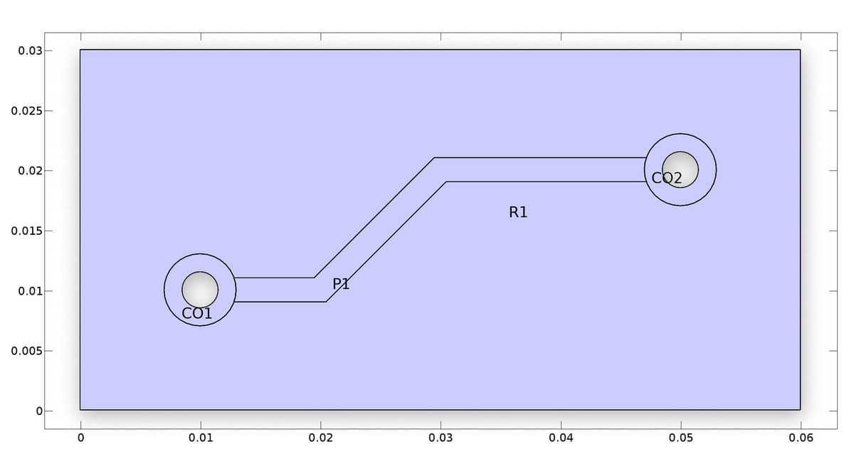
The first step is to define the two circles with inner and outer radii. Note that it is important to assign different name tags to the geometry objects (the last string input argument), so that there is no confusion when accessing and referring to them later.
ro = 0.003;   % Outer circle diameter.
ri = ro/2;    % Inner circle diameter.

% Circle 1.
co1 = gobj_circle( [0.01,0.01], ro, 'CO1' );
ci1 = gobj_circle( [0.01,0.01], ri, 'CI1' );

% Circle 2.
co2 = gobj_circle( [0.05,0.02], ro, 'CO2' );
ci2 = gobj_circle( [0.05,0.02], ri, 'CI2' );
The circular geometry objects are placed in the objects cell array of the main geom struct. This allows geometry operations to be performed on the geometry objects with the geom_apply_formula function. Here the inner circles are subtracted from the outer ones in order to create the two ring shapes.
% Remove inner holes from circles.
geom.objects = { co1 ci1 co2 ci2 };
geom = geom_apply_formula( geom, 'CO1-CI1' );
geom = geom_apply_formula( geom, 'CO2-CI2' );
A base rectangle r1 is defined, from which the solid outer circles are subtracted to make holes. Note that to do this the objects co1 and co2 are added back to the geom.objects field again (as they where already used to create the compound ring objects).
% Base rectangle.
r1 = gobj_rectangle( 0, 0.06, 0, 0.03, 'R1' );

% Remove (outer) circles from base rectangle.
geom.objects = [ geom.objects { r1 co1 co2 } ];
geom = geom_apply_formula( geom, 'R1-CO1-CO2' );
A polygon geometry object p1 is created for the conductive track. Again adding and removing the outer circles to create a well fitted object without overlap.
% Polygon for connecting conductive track.
w = 0.002/2;
p = [ 0.01   0.02-w/2 0.03-w/2 0.05   0.05   0.03+w/2 0.02+w/2 0.01   ;
      0.01+w 0.01+w   0.02+w   0.02+w 0.02-w 0.02-w   0.01-w   0.01-w ];
p1 = gobj_polygon( p', 'P1' );

% Remove outer circles from conductive track.
geom.objects = [ geom.objects { p1 co1 co2 } ];
geom = geom_apply_formula( geom, 'P1-CO1-CO2' );
The final step is to manually add and connect the rings to the track. This is to ensure that all objects are connected at minimum one boundary segment, which is not the case for the two rings (this last step will not be necessary in future FEATool versions).
% Join circles and conductive track.
geom = geom_apply_formula( geom, 'CS6+CS1+CS2' );
The plotgeom command can be used to plot and see the final geometry
plotgeom( geom )
2D Grid Generation
To create the initial 2D grid it is here recommended to use the external Triangle mesh generator as it is both significantly faster and also allows for better control over grid sizes. Here an average grid size hmax is chosen as half of the ring radii, with the first base subdomain 10 times larger, as a fine grid is not necessary outside of the conducting tracks.
hmax = (ro-ri)/2;
grid = gridgen_triangle( geom, 'hmax', [10*hmax hmax] );
Alternatively, if Triangle is not available it is also possible, although slower, to use the built-in gridgen function
grid = gridgen( geom, 'hmax', hmax );
The grid can be visualized with the plotgrid command
plotgrid( grid )
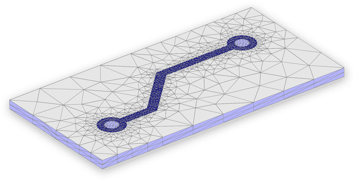
3D Grid Extrusion
Lastly, is to use the gridextrude function to extrude the unstructured 2D grid to 3D (here it is extruded a distance of 0.002 with a layer of 2 grid cells in the z-direction)
grid2 = gridextrude( grid, 2, 0.002 );
As above, the new grid and boundaries can be visualized with the plotgrid and plotbdr commands
plotgrid( grid2 )
plotbdr( grid2 )
To increase the resolution of the grid, one can either simply repeat the steps with a finer hmax value, or use the gridrefine function to create a uniform refinement.
It is also possible to import the grid into the FEATool GUI by using the Import > Variables From Main Workspace option from the File menu. Afterward, the internal FEATool GUI grid variable field can be overwritten by setting
fea.grid = grid2;
in the lower command prompt of the FEATool GUI Command Window. The complete gridextrude model script example is available from the link below