Gmsh Mesh Generator Integration
FEATool Multiphysics features full integration with the Gmsh grid and mesh generation software [1][2]. Both 2D and 3D GUI, and also MATLAB command line interface (CLI) use and MATLAB scripts are supported (with the gridgen and impexp_gmsh functions).
Advantages of using Gmsh compared to the built-in grid generation function is robustness and mesh generation speed (primarily for 3D geometries). Moreover, Gmsh also supports better and more control with a selection of different mesh generation algorithms, and specifying the grid size in different geometry regions, subdomains, as well as on boundaries, allowing for greater flexibility and better grids tuned for the specific problems and geometries. In addition Gmsh also supports generating boundary layers and unstructured quadrilateral grids in 2D.
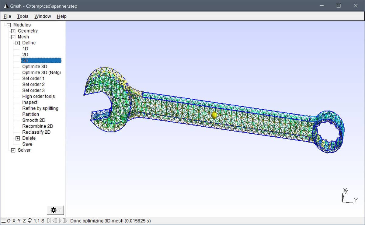
The gridgen function converts FEATool geometries to the Gmsh geo data file format via impexp_gmsh, makes a system call to Gmsh in non-interactive mode to generate a corresponding finite element FEM mesh, then parses, imports, and converts it back into a FEATool grid. For reference, as has been introduced previously, Gmsh can also be used to mesh and import CAD geometries to be used with FEATool.
Installation
First ensure that the latest FEATool Multiphysics version is installed with either MATLAB. If Gmsh has been selected but not found, FEATool will try to download, and install the mesh generator binary into the userpath/.featool folder.
Should the Gmsh installation fail, please manually download and install Gmsh from the original source reference (Gmsh versions 3.0.6, 4.3.0, and 4.5.2 are recommended as they have been tested and validated for use with FEATool) [1].
GUI Usage
Once installed, the Grid Generation Settings dialog box will in 2D and 3D feature a Gmsh selection option from the Grid Generation Algorithm drop-down box. Moreover, the following options also apply to the Gmsh mesh generation algorithm
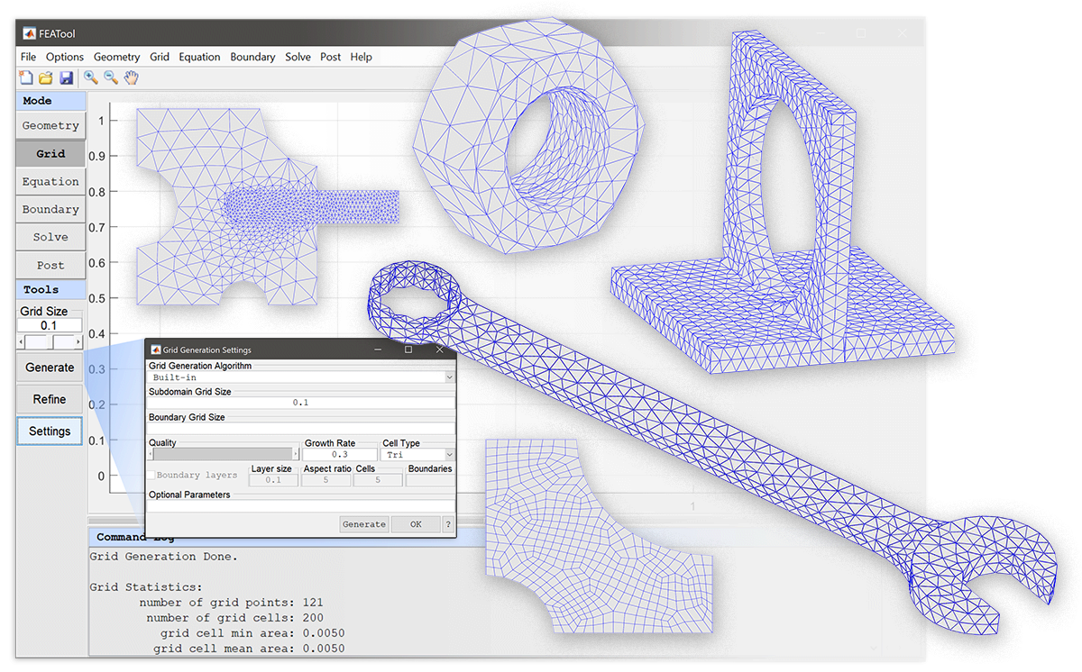
The Subdomain Grid Size, hmax, indicates the target grid cell diameter, and can either be a single scalar prescribing the grid size for the entire geometry, or a space separated string of numbers (array) where the hmax values correspond to the generated subdomains.
Boundary Grid Size, hmaxb, is analogous to hmax but related to boundaries (edges). hmaxb can consist of a single scalar applicable to all boundaries, for example
0.1prescribing a mean cell edge length of 0.1 on every boundary. hmaxb can also be a numeric array with entries corresponding to individual boundaries, for example
0.1 0.2 0.3 0.4specifying cell edge length 0.1 for boundary 1, 0.2 for boundary 2 etc.
The Smoothing parameter specifies the number of post grid smoothing steps to perform (default 3).
Selecting the Internal Boundaries checkbox in 2D enables mesh generation of structured boundary layers on boundaries. The height of the boundary layer can be specified with the Layer Size and also Aspect Ratio between cells. With Gmsh it is also possible to specify the number of mesh Cells in the boundary layer, and the boundary numbers to apply boundary layer generation to.
In 2D one can also choose between Triangular and Quadrilateral Cell Types.
The Generate grid button effectively calls the gridgen function from the GUI, which in turn makes a system call to Gmsh, after which the generated grid is automatically imported and displayed.
CLI Usage
On the MATLAB command line the gridgen function is used to call Gmsh to generate an unstructured 2D or 3D triangular grid. The following syntax is used
grid = gridgen( SIN, VARARGIN, 'gridgen', 'gmsh' )
where SIN is a valid FEATool fea problem struct, geometry struct, or cell array of geometry objects. gridgen also accepts the following property/value pairs (VARARGIN).
Property    Value/{Default}            Description
-----------------------------------------------------------------------------------
hmax        scal/arr {0.1}             Target grid size for geometry/subdomains
hmaxb       scal/arr {[]}              Target grid size for boundaries
nsm         scalar   {3}               Number of grid smoothing steps
nref        scalar   {0}               Number of uniform grid refinements
algo2       scalar   {2}               2D mesh algorithm (1=MeshAdapt, 2=Automatic,
                                       5=Delaunay, 6=Frontal, 7=BAMG, 8=DelQuad)
algo3       scalar   {1}               3D mesh algorithm (1=Del, 2=New Del, 4=Front
                                       5=Front Del, 6=Front Hex, 7=MMG3D, 9=R-tree)
blayer      struct   {[]}              Data struct for Gmsh 2D boundary layers
quad        boolean  {false}           Use quad meshing (for 2D)
tol         scalar   {eps*1e3}         Deduplication tolerance
compound    boolean  {true}            Use Gmsh compound boundaries
mshopt      cell     {}                Cell array of Gmsh options
mshall      boolean  {true}            Output/save all meshed entities
mshver      integer  {2}               Gmsh msh file version (1/2/4)
nt          integer  {numcores/2}      Number of concurrent threads
verbosity   integer  {5}               Gmsh verbosity/output level
syscmd      string   {'default'}       Gmsh system call command
                                       (default 'gmsh fdir/fname.geo -')
fname       string   {'fea_gmsh_UID'}  Gmsh imp/exp file name (root)
fdir        string   {tempdir}         Directory to write help files
clean       boolean  {true}            Delete (clean) Gmsh help files
instdir     string   {userpath/.featool}  Gmsh binary installation directory
fid         scalar   {1}               File identifier for output ([]=no output)
Among the properties hmax indicates target grid cell diameters, and is either a numeric scalar valid for the entire geometry or an array with hmax values corresponding to the subdomains. hmaxb is similar to hmax but a numeric array with a hmaxb values corresponding to the boundaries (including internal boundaries).
NSM (default 3) the number of post smoothing steps to perform. NREF (default 0) the number of post uniform grid refinement steps. ALGO2 and ALGO3 the Gmsh 2D and 3D mesh generation algorithms. QUAD (default 0) toggles Blossom-Quad conversion for 2D geometries.
Additional Gmsh options can be provided with the cell array MSHOPT.
For example MSHOPT could be given as {{‘Mesh’,
‘CharacteristicLengthMax’, ‘1’}, {‘Mesh’, ‘AnisoMax’, ‘10’}}
More detailed information regarding the mesh generation options can be found in the documentation for Gmsh [1]. Also, for more information about CLI usage access the function help by entering
>> help gridgen
in the MATLAB command line interface.
### Grid Generation Examples
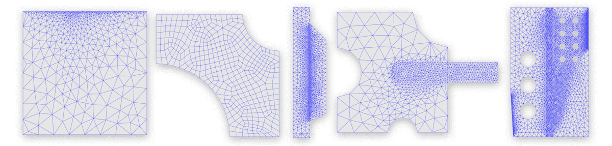
Unit square with uniform global grid size set to 0.1.
 grid = gridgen( {gobj_rectangle()}, 'hmax', 0.1, 'gridgen', 'gmsh' );
 plotgrid( grid )
Unit square with fine grid along the top boundary.
 grid = gridgen( {gobj_rectangle()}, 'hmax', 0.5, ...
                      'hmaxb', [0.5 0.5 0.01 0.5], 'gridgen', 'gmsh' );
 plotgrid( grid )
Domain with curved boundaries meshed with quadrilaterals.
 geom.objects = {gobj_rectangle() gobj_circle([0 0],.6) gobj_circle([1 1],.3,'C2')};
 geom = geom_apply_formula( geom, 'R1-C1-C2' );
 grid = gridgen( geom, 'hmax', 0.1, 'quad', true, 'gridgen', 'gmsh' );
 plotgrid( grid )
Two connected subdomains with refined grid along the shared boundary (9)
 geom.objects = { gobj_polygon([-2e-3 -8e-3;0 -8e-3;0 -6e-3;0 6e-3;0 8e-3;-2e-3 8e-3]), ...
                  gobj_polygon([0 -6e-3;2e-3 -5e-3;2e-3 4e-3;0 6e-3]) };
 hmax  = 5e-4;
 hmaxb = hmax*ones(1,4);
 hmaxb(9) = hmax/5;
 grid  = gridgen( geom, 'hmax', hmax, 'hmaxb', hmaxb, 'gridgen', 'gmsh' );
 plotgrid( grid )
Composite component with several subdomains.
 r1 = gobj_rectangle( 0, 0.11, 0, 0.12,  'R1' );
 c1 = gobj_circle( [ 0.065 0 ],   0.015, 'C1' );
 c2 = gobj_circle( [ 0.11 0.12 ], 0.035, 'C2' );
 c3 = gobj_circle( [ 0 0.06 ],    0.025, 'C3' );
 r2 = gobj_rectangle( 0.065, 0.16, 0.05, 0.07, 'R2' );
 c4 = gobj_circle( [ 0.065 0.06 ], 0.01, 'C4' );
 geom.objects = { r1 c1 c2 c3 r2 c4 };
 geom = geom_apply_formula( geom, 'R1-C1-C2-C3' );
 geom = geom_apply_formula( geom, 'R2+C4' );

 grid  = gridgen( geom, 'hmax', [0.0025 0.05 0.0025], 'gridgen', 'gmsh' );
 plotgrid( grid )
Complex geometry with several holes and subdomains.
 w = 10e-4; L = 3*w; H = 5*w;
 p1  = gobj_polygon( [w/10 0;(L-w/4)/2 0;(L-w/4)/2 H;0 H;0 H/3], 'P1' );
 p2  = gobj_polygon( [(L+w/4)/2 0;L 0;L H-H/3;L H;(L+w/4)/2 H], 'P2' );
 r1  = gobj_rectangle( (L-w/4)/2, (L+w/4)/2, 0, H, 'R1' );
 c1  = gobj_circle( [2*w/3 3*w], w/3, 'C1' );
 c2  = gobj_circle( [2*w/3 2*w], w/3, 'C2' );
 c3  = gobj_circle( [2*w/3 1*w], w/3, 'C3' );
 c4  = gobj_circle( [L-w/2 4.5*w], w/8, 'C4' );
 c5  = gobj_circle( [L-w   4.5*w], w/8, 'C5' );
 c6  = gobj_circle( [L-w/2 4*w], w/8, 'C6' );
 c7  = gobj_circle( [L-w   4*w], w/8, 'C7' );
 c8  = gobj_circle( [L-w/2 3.5*w], w/8, 'C8' );
 c9  = gobj_circle( [L-w   3.5*w], w/8, 'C9' );
 c10 = gobj_circle( [L-w/2 3*w], w/8, 'C10' );
 c11 = gobj_circle( [L-w   3*w], w/8, 'C11' );

 geom.objects = { p1 p2 r1 c1 c2 c3 c4 c5 c6 c7 c8 c9 c10 c11 };
 geom = geom_apply_formula( geom, 'P1-C1-C2-C3' );
 geom = geom_apply_formula( geom, 'P2-C4-C5-C6-C7-C8-C9-C10-C11' );

 hmaxb = zeros(1,21);
 hmaxb([6 20]) = w/50;
 grid = gridgen( geom, 'hmax', w./[5 20 5], 'hmaxb', hmaxb, 'gridgen', 'gmsh' );
 plotgrid( grid )
Usage Notes
For geometries with multiple and overlapping geometry objects the actual subdomain numbering will generally not correspond to the geometry object numbering (two intersecting geometry objects will for example create three or more subdomains and several internal boundaries). In this case the actual subdomain and boundary numbering for vector valued hmax and hmaxb arrays can easiest be visualized and determined by first creating a coarse grid and switching to Equation/Subdomain and Boundary modes, respectively.
Gmsh propagates the hmax and hmaxb values down to the specific nodes in the mesh which means that it is currently not possible to exactly define mesh sizes for subdomains and boundaries.
The temporary Gmsh generated geo and msh data files can be found in the specified fdir directory (default given by the MATLAB tempdir function).
References
[1] Gmsh home page - A three-dimensional finite element mesh generator with built-in pre- and post-processing facilities.
[2] C. Geuzaine and J.-F. Remacle. Gmsh: a three-dimensional finite element mesh generator with built-in pre- and post-processing facilities. International Journal for Numerical Methods in Engineering 79 (11), pp. 1309-1331, 2009.