The Plotly javascript plotting and visualization library is now fully integrated with FEATool Multiphysics and can be used to visualize FEM simulation results and data. In comparison with the built-in MATLAB graphics, plotly plots feature the following advantages
- fully self-contained and interactive web graphics pages
- high performance plots with further export functionality
- share with coworkers and colleagues through cloud and web services
Plotly plots are stand-alone html web pages that can be inspected, rotated, zoomed, and exported as image and svg files. Moreover, as the plots are self-contained, including the embedded plotly javascript library, they can be more easily shared during collaborative projects rather than large binary simulation data files. The FEATool-Plotly postprocessing functionality supports all standard finite element FEM plotting options such as surface, contour, height, iso, and arrow plots in 1D, 2D, and 3D.
Plotly MATLAB GUI Usage
Plotly plots can easily be created directly from within the GUI by simply clicking one of the buttons labeled Plotly, either in the postprocessing toolbar or in the postprocessing settings dialog box. The currently selected plot options will be exported as plotly visualization data and saved to a corresponding html text file.
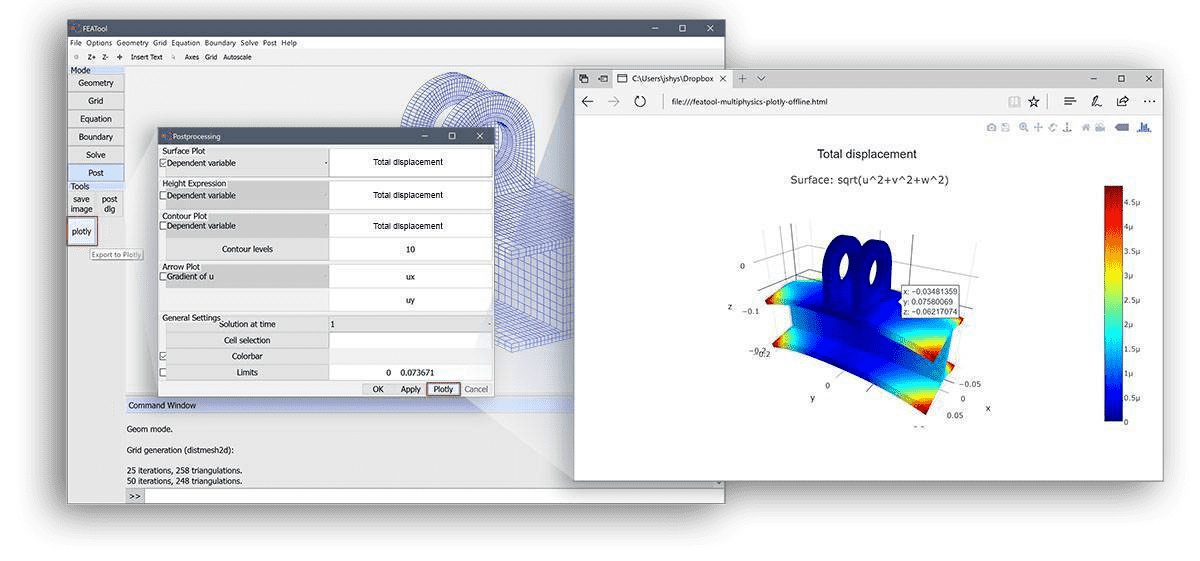
The newly created plotly plot will automatically be opened in the default system web browser where the plot and data can then be examined with the plotly interface, exported as image files, and also uploaded to the plotly cloud for sharing and collaboration (see for example the FEATool Multiphysics Plotly plot examples).
Plotly MATLAB CLI Usage
MATLAB CLI command line usage with plotly is just as easy
as using the normal postprocessing functions and commands. The
postplot function (type
help postplot for a usage help and list input arguments)
includes a renderer flag with a plotly option. To use plotly
simply add this flag to a corresponding postplot command
postplot( fea, ..., 'renderer', 'plotly' )
where … denotes the usual postprocessing property value pairs such as surfexpr, isoexpr, and arrowexpr etc. The plotly postprocessing MATLAB json data struct can also optionally be obtained as output
plotly_data = postplot( fea, ..., 'renderer', 'plotly' );
and corresponding web html file generation can manually be called with
html_file = plotlyoffline( plotly_data );
where html_file is a string containing the name of the plotly output file (default featool-multiphysics-plotly-offline.html in the current directory)
Plotly Structural Mechanics Postprocessing Example
For example, the image above, depicting the structural mechanics (SME) displacements for an I-beam as a full 3D surface plot, can be created with the following m-script commands in MATLAB
% Set up model, solve, and return element fea/fem data.
fea = ex_linearelasticity4( 'ilev', 1 );

% Optionally deform grid according to displacement.
dscale = 5e3;
dp = zeros(size(fea.grid.p));
for i=1:3
  dp(i,:) = dscale * evalexpr( fea.dvar{i}, fea.grid.p, fea );
end
fea.grid.p = fea.grid.p + dp;

% Postprocessing call with 'plotly' renderer flag.
postplot( fea, 'surfexpr', 'sqrt(u^2+v^2+w^2)', ...
               'title',    'Total displacement', ...
               'renderer', 'plotly' )
The following link shows the generated web plot (note that it might take a few seconds to load due to the included plotly js-library)
Note, that the Plotly web plot is fully interactive, that is if mouse pointer or cursor moved above the plot one can zoom in, zoom out, rotate, pan, inspect coordinates and values, export the plot in different formats, and also save it online to the plotly cloud.
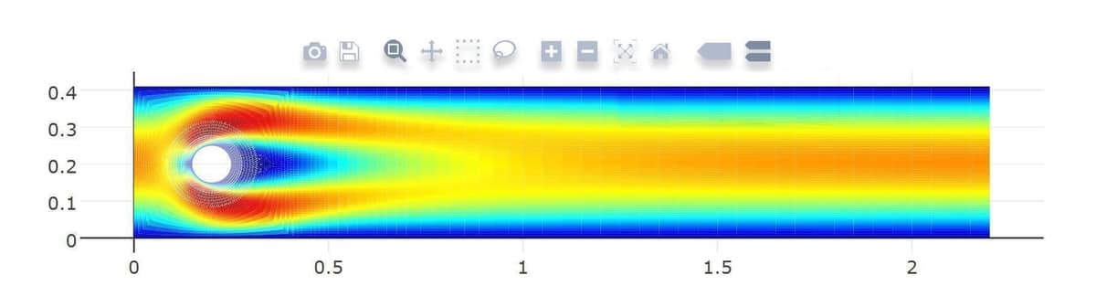
Plotly Fluid Dynamics CFD Postprocessing Example
The following short command line script examples show how to create 2D surface plot CFD visualizations with plotly. The first step is to create the simulation data, in this case the pre-defined CFD cylinder flow benchmark model example is used
% Create finite element fea model and result data.
fea = ex_navierstokes3();
The generated mesh and grid can then be visualized with the
plotgrid function
as
plotgrid( fea, 'renderer', 'plotly' )
In addition to supporting the postplot and plotgrid commands, the renderer plotly flag is also supported by the plotsubd and plotbdr functions (to visualize geometry boundaries and subdomains).
Furthermore, the following command visualizes the velocity field magnitude as surface data, pressure as contour lines, and velocity field field as arrows
postplot( fea, 'surfexpr', 'sqrt(u^2+v^2)', ...
               'isoexpr', 'p', ...
               'arrowexpr', {'u' 'v'}, ...
               'renderer', 'plotly' )
It is easy to compare the plotly visualizations with MATLAB by just omitting the renderer flag. Further information on postprocessing options and using plotly with FEATool can be found in the postprocessing section of the FEATool User’s Guide.
As has been described, it is now easy and straightforward to create good looking and interactive simulation web plots, visualizations, and graphics with the built-in plotly functionality. External data, not generated with FEATool, is also possible to import and convert to visualize and postprocess with plotly and the postplot functionality. The linked article discusses how to do postprocessing and importing data from unstructured grids.
Please try out the FEATool-Plotly visualization and share your models and multiphysics FEM simulation plots.