This post explains how to use MATLAB and the FEATool postprocessing function library to import, plot, and visualize general data on unstructured grids and meshes. Although MATLAB do include visualization functionality for surface and contour plots (with the surf and contour functions), it is currently limited to regular structured tensor-product grids (such as those created with meshgrid). As detailed below, in this case one can then easily make use of FEATool postprocessing functions to plot surface, height, arrow, and contour plots even for external non-FEATool or general non finite element analysis FEM data.
Unstructured Grid and Data Import
The first processing step is to import the unstructured grid data and convert it to FEATool format. The FEATool grid and mesh format is described in the grid reference section of the FEATool User’s Guide. FEATool includes several built-in functions for importing and exporting grid and mesh files from external grid generation tools and formats such as GiD, Gmsh, and XML. An tutorial showing how to import grids from text files can be found in the corresponding grid import and export section. Moreover, it is straight forward to convert pure ASCII grid data to FEATool format from just having access to the grid point vertices or coordinates and grid cell connectivities.
For example, here a random distribution of points is used with a Delaunay triangulation, however, importing grid data from external files would proceed similarly
grid.p = rand(2,100);            % 2d random distribution of 100 points.
grid.c = delaunay( grid.p' )';   % Delaunay triangulation for grid cell connectivities.
Having the grid point vertices and connectivities one can use the grid
utility functions gridadj
and gridbdr to reconstruct
the other grid data struct fields
grid.a = gridadj( grid.c, size(grid.p,1) );   % Grid cell adjacency.
grid.b = gridbdr( grid.p, grid.c, grid.a );   % Grid boundary data.
grid.s = ones(1,size(grid.c,2));              % Set subdomain number 1 for all cells.

fea.grid = grid;                              % Assign grid to fea struct.
fea.sdim = {'x' 'y'};                         % Assign space dimension coordinate names.
After the grid has been imported and extended one can proceed with
importing the unstructured data to be visualized. If the data is
available in ASCII, CSV, or MATLAB binary mat file format, then
one can simply use the load filename.txt command and the
data will be loaded into a variable in the main workspace labeled
filename.
Data to FEA Struct Conversion
The data must now be converted and reshaped to FEATool solution vector format which is specified as a column vector of size nvars*np x 1, where np is the number of grid points and nvars the number of variables to visualize. That is, the solution or visualization vector should conform to nvars vertically stacked column vectors, where each block with contains variable data corresponding to the grid points.
Continuing the example, assuming that two visualization variables have been loaded, the first with sin(x) coordinates and the second with y^2 values (instead of loading and importing they are for simplicity constructed directly here)
u1 = sin( grid.p(1,:) )';
u2 = grid.p(2,:).^2';

fea.sol.u = [u1;u2];   % Assign variables to solution vector.
In order to use and apply FEATool postprocessing and plotting functions to these variables they must first be represented as finite element FEM dependent variables or unknowns (solving for them is not necessary as they are only used for visualization)
fea.dvar = {'u' 'v'};
fea.sfun = repmat({'sflag1'},1,length(fea.dvar));
The dvar field is the name string or tag used to access and call the variables in the postprocessing functions. The sfun field represents the finite element shape function, and in this case node oriented linear first order P1 functions (sflag1) are prescribed, as is appropriate when the imported visualization data is defined in the grid points or nodes. As can be seen one will need to assign one dvar name and sfun entry for each imported data block (equal to the number of stacked column blocks in the solution vector fea.sol.u).
Posprocessing with FEATool Plot Functions
To enable FEATool postprocessing the parseprob function is first
called to automatically generate some additional fields such as
degrees of freedom maps. Now it is possible to use the created fea
finite element data struct with imported unstructured data in
postprocessing with for example the
postplot function
fea = parseprob( fea );
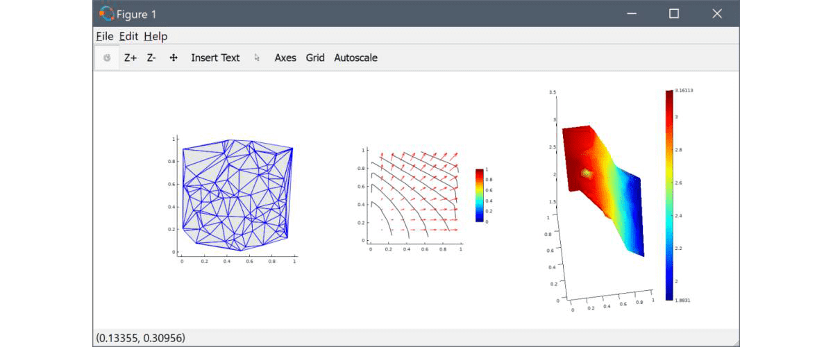
% Plot grid.
subplot(1,3,1)
plotgrid( fea )
% Plot iso-contour lines 'u+v' and arrows 'u' and 'v'.
subplot(1,3,2)
postplot( fea, 'isoexpr', 'u+v', 'arrowexpr', {'u' 'v'} )
% Plot height surface expression 'pi*du/dx'.
subplot(1,3,3)
postplot( fea, 'surfexpr', 'pi*ux', 'surfhexpr', 'pi*ux' )
Note, that the imported data has here been assigned as general finite element solution variables. In this way they can be included in general FEATool expressions (for example expressions such as 1+u^2+x*sin(v)) and also processed like ux for the first derivative (which is computed from the first order finite element basis function approximation). Thus having imported the data into FEATool FEM format one is not limited to the data as is, but can process it using the full FEATool functionality.
One can for example also perform boundary and subdomain integration, and general expression evaluation in any coordinates like
% Evaluate expression 2*x+sqrt(ux^2+vy^2) at p.
p = [0.1 0.8;0.2 0.3];   % Evaluation coordinates.
val = evalexpr( '2*x+sqrt(ux^2+vy^2)', p, fea )
In addition to creating plots in MATLAB it is also possible to use the the Plotly functionality to create and export interactive web and html graphics and plots as described in the plotly FEATool tutorial article.
Lastly, if desired one can import the created fea data struct into the FEATool GUI and use the GUI postprocessing functionality instead of working on the command line. This can be done by starting a new FEATool model with the same space dimensions as the data, switching to Postprocessing mode, and using the Import > Variables From Main Workspace… File menu option.