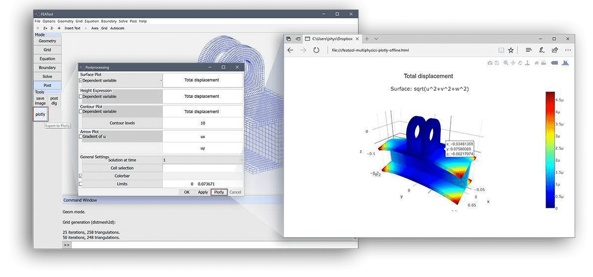
FEATool can be used to easily generate interactive surface, contour, arrow, and other visualizations of unstructured mesh and simulation data in 1D, 2D, and 3D. As FEATool also supports Plotly as rendering and visualization engine it is possible to create, interactively explore, and share simulation and unstructured data directly on the web. This post explains and gives examples how fully three-dimensional (3D) visualizations can be created using the MATLAB CLI interface together with FEATool and Plotly.

(Please note that due to loading the Plotly JS library and interactive plot data the responsiveness of this page can be delayed.)

Unstructured Grid and Data Import

FEATool is a fully integrated multiphysics simulation toolbox, however, in the following only the FEATool postprocessing functionality will be used on imported external data. Moreover, although one can just as easily use the graphical user interface (GUI), the examples are shown using the MATLAB CLI interface which can be scripted for automatic processing.

Plotly Visualization with the FEATool GUI

The first processing step is to import the unstructured grid or mesh data and convert it to FEATool format. The FEATool grid and mesh format is quite simple and fully described in the grid reference section of the FEATool User’s Guide. Moreover, FEATool includes several built-in functions for importing and exporting grid and mesh files from external grid generation tools and formats such as GiD, Gmsh, and XML. It is also straight forward to convert pure ASCII grid data to FEATool format from just having access to the grid point vertices or coordinates and grid cell connectivities. A tutorial showing how to import grids from text files can be found in the corresponding grid import and export section.

Instead of importing a mesh, here for simplicity we will manually construct a grid of overlapping cylinders to have something interesting to look at, and generate corresponding vertex data consisting of the distance from the center lines to the cylinder walls. The following m-script commands achieves this (but again this will not be necessary if data is imported)

% Point distribution.
n_p = 18;   % Number of radial points.
n_z = 20;   % Number of points lengthwise.
th = linspace(0,2*pi,n_p);
p = [];
for r=[0.05 0.1 0.2 0.3];
  for z_i=linspace(-1,1,n_z)
    p = [ p; [ r*cos(th(1:end-1)) z_i*ones(1,n_p-1)  r*sin(th(1:end-1)) ;
               r*sin(th(1:end-1)) r*cos(th(1:end-1)) z_i*ones(1,n_p-1)  ;
               z_i*ones(1,n_p-1)  r*sin(th(1:end-1)) r*cos(th(1:end-1)) ]' ];
  end
end

% Triangulate points.
t = delaunay( p );

% Remove triangulated cells outside the cylinders.
pc = [ mean( reshape( p(t,1), size(t) )' )' ...
       mean( reshape( p(t,2), size(t) )' )' ...
       mean( reshape( p(t,3), size(t) )' )' ];   % Cell center coordinates.
t = t( any( [ sqrt( pc(:,1).^2 + pc(:,2).^2 )' ;
              sqrt( pc(:,1).^2 + pc(:,3).^2 )' ;
              sqrt( pc(:,2).^2 + pc(:,3).^2 )' ] <= r+sqrt(eps) ), : );

% Generate distance function distribution.
u = min([ sqrt( p(:,1).^2 + p(:,2).^2 )' ;
          sqrt( p(:,1).^2 + p(:,3).^2 )' ;
          sqrt( p(:,2).^2 + p(:,3).^2 )' ])';
p = p'; t = t';   % Transpose to change to row ordering.

Here, the variables p, t, and u now contain the grid points, triangulation, and data.

Grid and Mesh Struct

The generated, imported, or simulated grid and data can now be used to define a FEATool grid and FEA data struct, which in turn can be used by the postprocessing functions. A grid struct can be created with the following MATLAB commands

grid.p = p;   % Grid/mesh points.
grid.c = t;   % Grid/mesh cells.

Having the grid point vertices and connectivities one can use the grid utility functions gridadj and gridbdr to reconstruct the necessary adjacency, boundary, and subdomain fields

grid.a = gridadj( grid.c, size(grid.p,1) );   % Grid cell adjacency.
grid.b = gridbdr( grid.p, grid.c, grid.a );   % Grid boundary data.
grid.s = ones(1,size(grid.c,2));              % Set subdomain number 1 for all cells.

Now, with the complete grid struct we can simply plot the grid with

plotgrid( grid )

which displays a MATLAB figure with the grid. Optionally, we can add the plotly renderer property to instead generate a plotly visualization.

(Note that the following plots are fully interactive Plotly visualizations which can be rotated, zoomed, and inspected.)

plotgrid( grid, 'renderer', 'plotly' )

Data FEA Struct

In order to use and apply FEATool postprocessing and plotting functions to these variables they must first be represented as finite element FEM dependent variables or unknowns (solving for them is not necessary as they are only used for visualization).

The grid is simply stored in the corresponding grid field, while sdim represents the names of the space dimensions. The dvar field is the name string or tag used to access and call the variables in the postprocessing functions. Lastly, the sfun field specifies the finite element shape function, in this case node oriented linear first order P1 functions (sflag1) are prescribed, which is appropriate when the imported visualization data is defined in the grid points or vertex nodes.

% Define help fea finite element struct.
fea.grid = grid;            % Assign grid to fea struct.
fea.sdim = {'x' 'y' 'z'};   % Assign space dimension coordinate names.
fea.dvar = {'u'};           % Assign help dependent variable name.
fea.sfun = {'sflag1'};      % Assign linear interpolation.

The imported or generated data must now be converted and reshaped to a column vector format which is specified as a column vector of size np x 1, where np is the number of grid points. Moreover, the fea struct is checked, validated, and parsed to be able to be used by the postplot function.

% Check and parse fea struct and assign solution data field.
fea.sol.u = u(:);
fea = parseprob( fea );

Postprocessing and Visualization

With the FEATool fea struct complete, we can now use the postplot function to visualize the data. Moreover, volume and boundary integration, and arbitrary point evaluation is also possible since we represent the data as a continuous finite element solution. The following are some examples of visualizations that can be made.

Surface Plot

A surface plot of a general expression, here u+sin(2pix)

postplot( fea, 'surfexpr', 'u+sin(2*pi*x)', ...
               'renderer', 'plotly' )

In FEATool, valid string expressions may be functions of the data itself u, space dimensions x, y, z, built-in MATLAB functions (sin, log, etc.), custom user defined functions on the MATLAB path, and even first and second derivatives of the data (expressed as for example ux and uyy). In this way complex visualization and postprocessing expressions are conveniently parsed automatically by FEATool, and do not require the user to explicitly calculate them.

Slice and Arrow Plots

Here we plot the computed distance from the center lines, u, as slices and add arrows for the corresponding derivative (FEATool automatically computes this when using the ux, uy, and uz expressions).

postplot( fea, 'sliceexpr', 'u', ...
               'arrowexpr', {'ux' 'uy' 'uz'}, ...
               'arrowspacing', [25 25 25], ...
               'renderer', 'plotly' )

Iso-surface Plot

The iso-surface functionality is somewhat coarse, as it interpolates to a background grid, the example here nevertheless illustrates the logical switch expression concept. Here by plotting _u*(z<0)_ everyting in the upper half plane is simply canceled out (evaluated to zero)

postplot( fea, 'isoexpr', 'u*(z<0)', ...
               'isolev', 5, ...
               'renderer', 'plotly' )

Although these examples have been for full 3D visualizations, 1D and 2D is similarly supported as the two-dimensional unstructured MATLAB surface and contour plots illustrated here.