Periodic Boundary Conditions and the Solver Hook Functionality

This post describes how to implement finite element FEM models with custom periodic boundary conditions in FEATool. A periodic boundary condition can be defined for opposing boundaries so that their values are linked in some defined way. The typical case for two periodic boundaries is to require them to have identical values, thus representing a partly infinite domain. They can also be used to offset boundary values by a constant, such as for flow boundaries with a given pressure differential.

As periodic boundary conditions are currently not part of the pre-defined physics modes, they have to be implemented by custom modifications. This can be accomplished with the solver hook functionality described below.

Solve Hook Functionality

The solver hook functionality is a part of the solvestat and solvetime functions to allow for custom matrix and right hand side vector modifications. The functionality can currently only be activated for Neumann boundary conditions defined with a string coefficient named solve_hook_myfun (where myfun can be any custom function name). This is also applicable to the MATLAB GUI for physics modes where pure Neumann boundary coefficients can be prescribed. If present, the solver will discard the solve_hook_ prefix and try to call the function myfun both before and after the linear solver calls (u = A\b). The solve hook function header and calls take the form

function [ A, f, fea ] = myfun( A, f, fea, i_dvar, j_bdr, solve_step )

where A and f are the assembled system matrix and right hand side/load vector, respectively. fea is the finite element problem struct, i_dvar the current dependent variable, j_bdr the boundary. solve_step is an integer flag which indicates if the call is before the linear solve step (1), or after it (2). The (optionally) modified outputs are returned in A, f, and fea. In pseudo code the solve hook calling step looks something like the following

...

if( exist('myfun') )
  [A,f,fea] = myfun( A, f, fea, i_dvar, j_bdr, 1 );
end

u = A\f;

if( exist('myfun') )
  [A,f,fea] = myfun( A, f, fea, i_dvar, j_bdr, 2 );
end

...

Besides being used to set and apply periodic boundary conditions as explained below, the solve hook functionality is also automatically used to set velocity slip boundary conditions (non-aligned with the coordinate system) for Navier-Stokes and Brinkman equation fluid flow physics modes, and can also to couple dependent variables between different active subdomains and physics modes.

Moving Pulse with Periodic Boundary Conditions

This example shows how to use the solve hook functionality to define a periodic pulse that is moving out from one side of a one dimensional domain and reentering the other. The first step to define the model on the command line is to assign a name or label for the space dimension (here x), and generate a 100 cell grid for the unit line

fea.sdim = {'x'};
fea.grid = linegrid( 100 );

Next, the convection and diffusion physics mode is added with a diffusion coefficient of 1, and a constant convection velocity of 0.002 in the forward x-direction

fea = addphys( fea, @convectiondiffusion );
fea.phys.cd.eqn.coef{3,end} = { 1 };
fea.phys.cd.eqn.coef{2,end} = { 0.002 };
fea = parsephys( fea );

The parsephys call processes the physics mode and translates the information to the global finite element fea.eqn and fea.bdr fields.

Proceeding, any prescribed Dirichlet boundary conditions are cleared (which if present take priority over and overrides Neumann flux boundary conditions), and a solve_hook function, here named periodic_bc, is prescribed for the right node (boundary 2).

i_dvar = 1;   % Dependent variable number.
j_bdr  = 2;   % Boundary selection.

fea.bdr.d{i_dvar} = { [] [] };
fea.bdr.n{i_dvar}{j_bdr} = 'solve_hook_periodic_bc';

Before the problem can be solved, the actual periodic_bc function must first be created and defined. To do this, create a separate file named periodic_bc.m with the following contents

function [ A, f, prob ] = periodic_bc( A, f, prob, i_dvar, j_bdr, solve_step )

% Only process step before the linear solver call.
if( solve_step~=1 ), return, end

% Sparsify matrix if necessary.
if( isstruct(A) ), A = sparse( A.rows, A.cols, A.vals, A.size(1), A.size(2) ); end

% Degrees of freedom to couple.
dof_i = 1;               % Left side node/dof.
dof_j = prob.eqn.ndof;   % Right side node/dof.

% Add i and j rows (to preserve both i and j equations).
A(dof_i,:) = A(dof_i,:) + A(dof_j,:);
f(dof_i)   = f(dof_i)   + f(dof_j);

% Modify j rows so that A(j,i) - A(j,j) = 0.
A(dof_j,:) = 0;   % Zero out periodic bc rows.
A(dof_j,[dof_i dof_j]) =  [ 1 -1 ];
f(dof_j) = 0;

The periodic_bc function is here customized for this exact problem to couple the first (left side) node (degree of freedom) with the last right side one. In essence this modifies the A matrix so that the relation u(1) - u(100) = 0 is enforced.

Finally, assuming the periodic_bc function exists and can be found in any of the the MATLAB paths, the problem can now be checked for error, parsed, and solved with a unit pulse defined between x=0.4 and x=0.6

fea = parseprob( fea );
fea.sol.u = solvetime( fea, 'init', '(x>=0.4)*(x<=0.6)', ...
                       'tstep', 0.005, 'tmax', 1 );

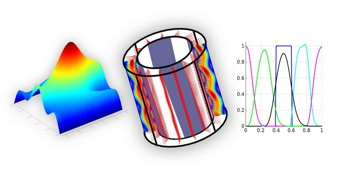
After the solver has finished, the solution at different times can be plotted and visualized with the following code

postplot( fea, 'surfexpr', 'c', 'solnum', 1, 'color', 'b' )
postplot( fea, 'surfexpr', 'c', 'solnum', floor(size(fea.sol.u,2)/4), 'color', 'c' )
postplot( fea, 'surfexpr', 'c', 'solnum', floor(size(fea.sol.u,2)/2), 'color', 'm' )
postplot( fea, 'surfexpr', 'c', 'solnum', floor(size(fea.sol.u,2)*3/4), 'color', 'g' )
postplot( fea, 'surfexpr', 'c', 'solnum', size(fea.sol.u,2) )
axis( [0 1 0 1] )
grid on

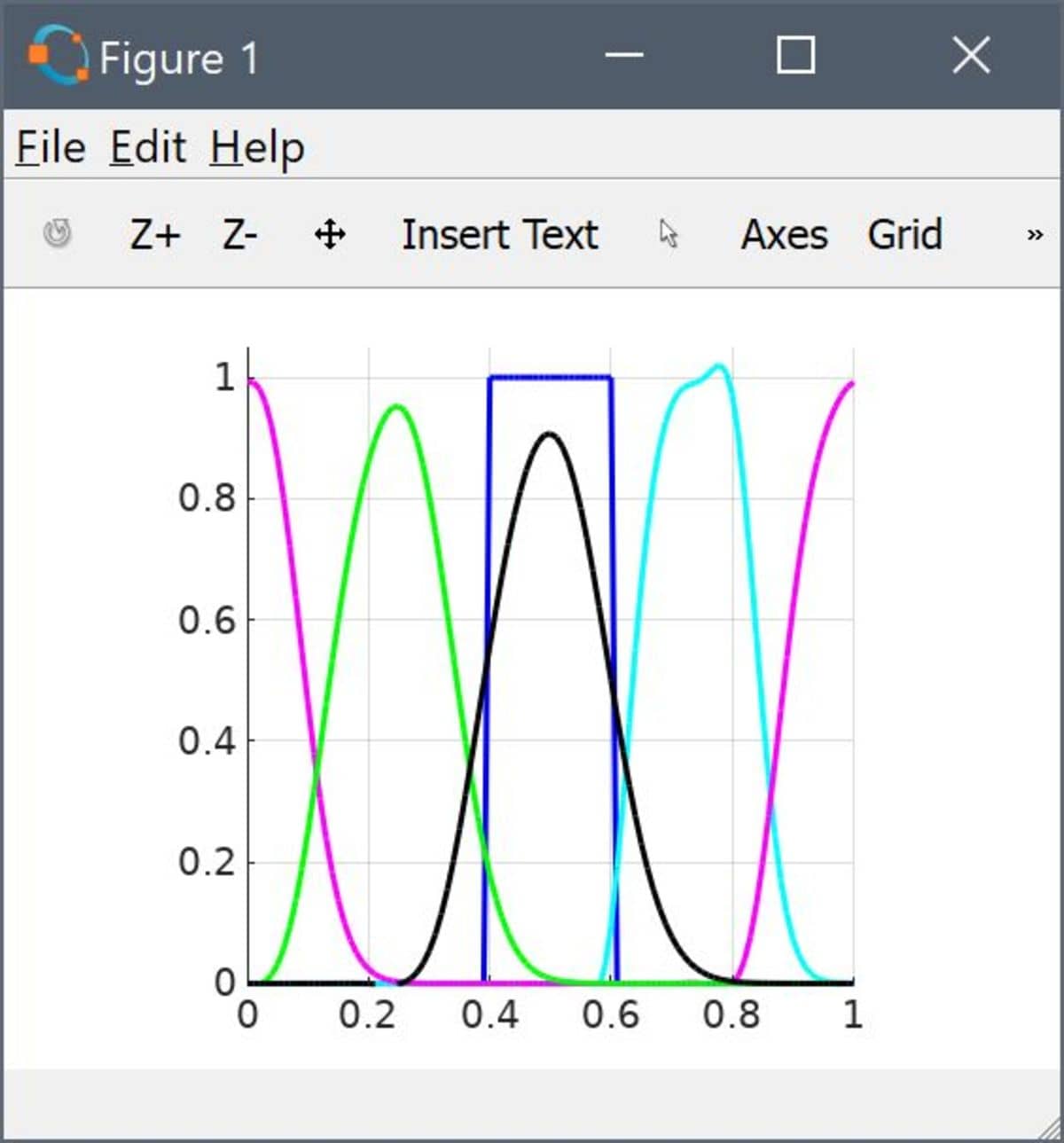
Alternatively, snapshots and an animated gif movie of the moving pulse can be created with these commands (assuming that the convert tool from ImageMagick is installed)

x = linspace(0,1,101);
for i=1:size(fea.sol.u,2)
  y = fea.sol.u(:,i); clf
  patch( 'vertices', [[0;x(:);1] [0;y(:);0]], 'faces', [1:103 1], ...
         'facecolor', [0.5 0.5 0.8], 'linewidth', 3 );
  set( gca, 'fontsize', 20, 'ytick', [], 'ycolor', [1 1 1] )
  axis( [0 1 0 1.05] )
  print( '-r200', '-dpng', sprintf( 'img%03i.jpg', i ) )
end

system( ['convert -loop 0 img*.png -resize 640x480 -dither none' ...
         '-colors 8 -fuzz "40%" -layers OptimizeFrame output.gif'] )

As can be seen the solution depicts an initially square pulse being smoothed due to diffusion while moving to the right. As it reaches the right hand side edge it reenters the left side as expected from a periodic domain.

Other Periodic Boundary Condition Examples

For more examples defining and using periodic boundary the conditions, see the axisymmetric Taylor-Couette swirl flow model, and the two dimensional periodic Poisson equation example which is available in the FEATool model and examples directory as the ex_periodic2 MATLAB script file.