Orthotropic Heat Conduction

This is an example of modeling anisotropic heat conduction in an orthotropic material where a heated solid bar suddenly is cooled by submerging it in a cool fluid. The material features different thermal conductivities in the x and y-directions which is accounted for by modifying the diffusion term in the heat transfer equation. Instead of solving the usual isotropic case

we will instead solve the following

where $$ = 34.6147 and $$ = 6.23687 W/mK are the thermal conductivities in the different directions. Fully anisotropic cases can technically also be handled by introducting off-diagonal $$ diffusion terms.

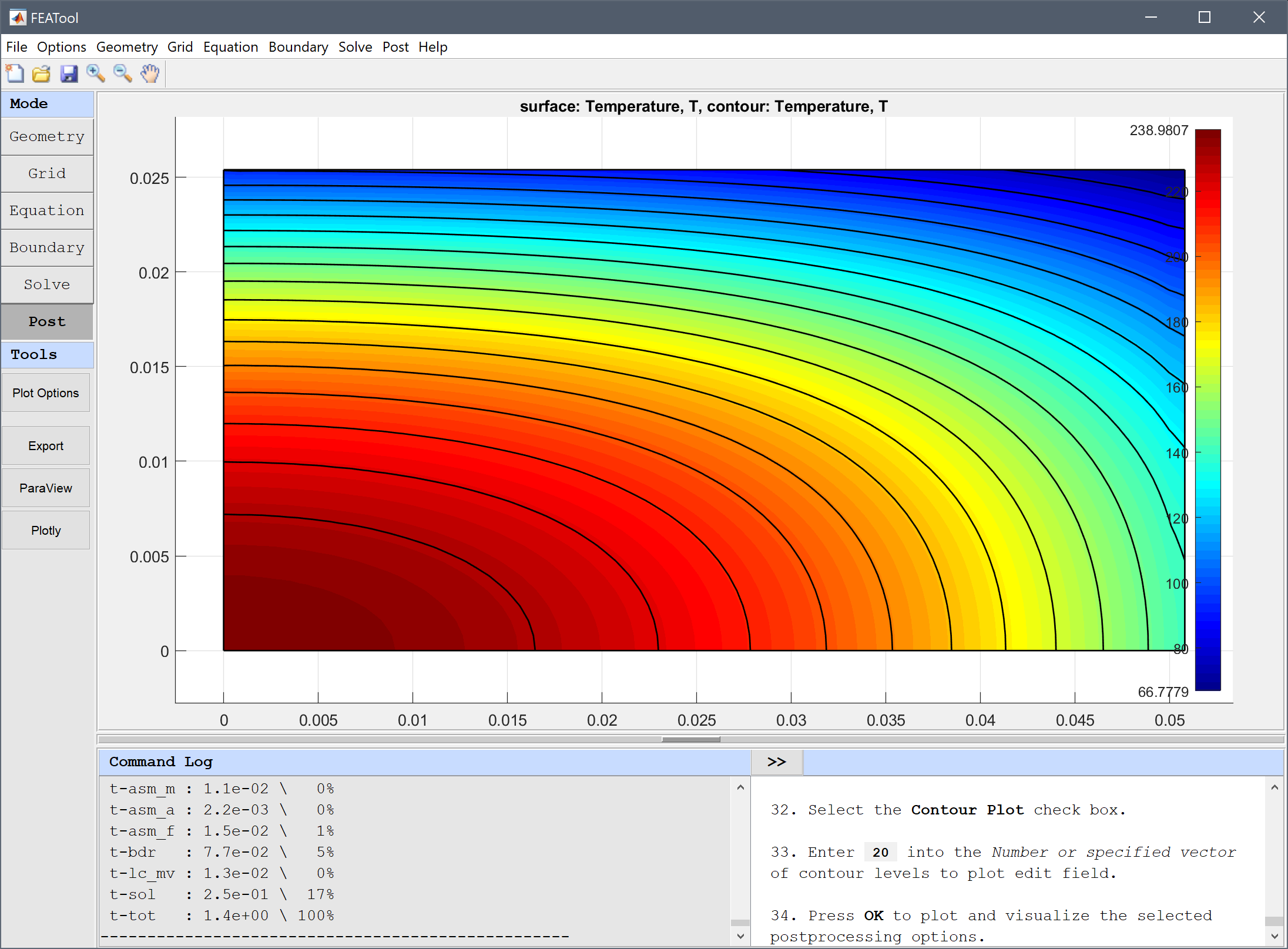
The following material and simulation parameters are given; initial temperature T₀ = 260 °C, density ρ = 6407.4 kg/m³, heat capacity $$ = 37.688 J/kgK. Due to symmetry we only need to model a quarter domain of a 2D cross-section with dimensions 5.08 by 2.54 cm. Conductive heat flux boundary conditions are used on the external boundaries with a convection coefficient h = 1361.7 W/m²K and surrounding temperature T_inf = 37.7778 °C. The cooling process is simulated for 3 seconds after which the temperature is measured in the center core and corners, and compared to the reference values [1].

This model is available as an automated tutorial by selecting Model Examples and Tutorials… > Heat Transfer > Orthotropic Heat Conduction from the File menu. Or alternatively, follow the linked step-by-step instructions.

Reference

[1] P.J. Schneider, Conduction Heat Transfer, Addison-Wesley, 2nd Ed., Ex. 10-7, pp. 261, 1957.