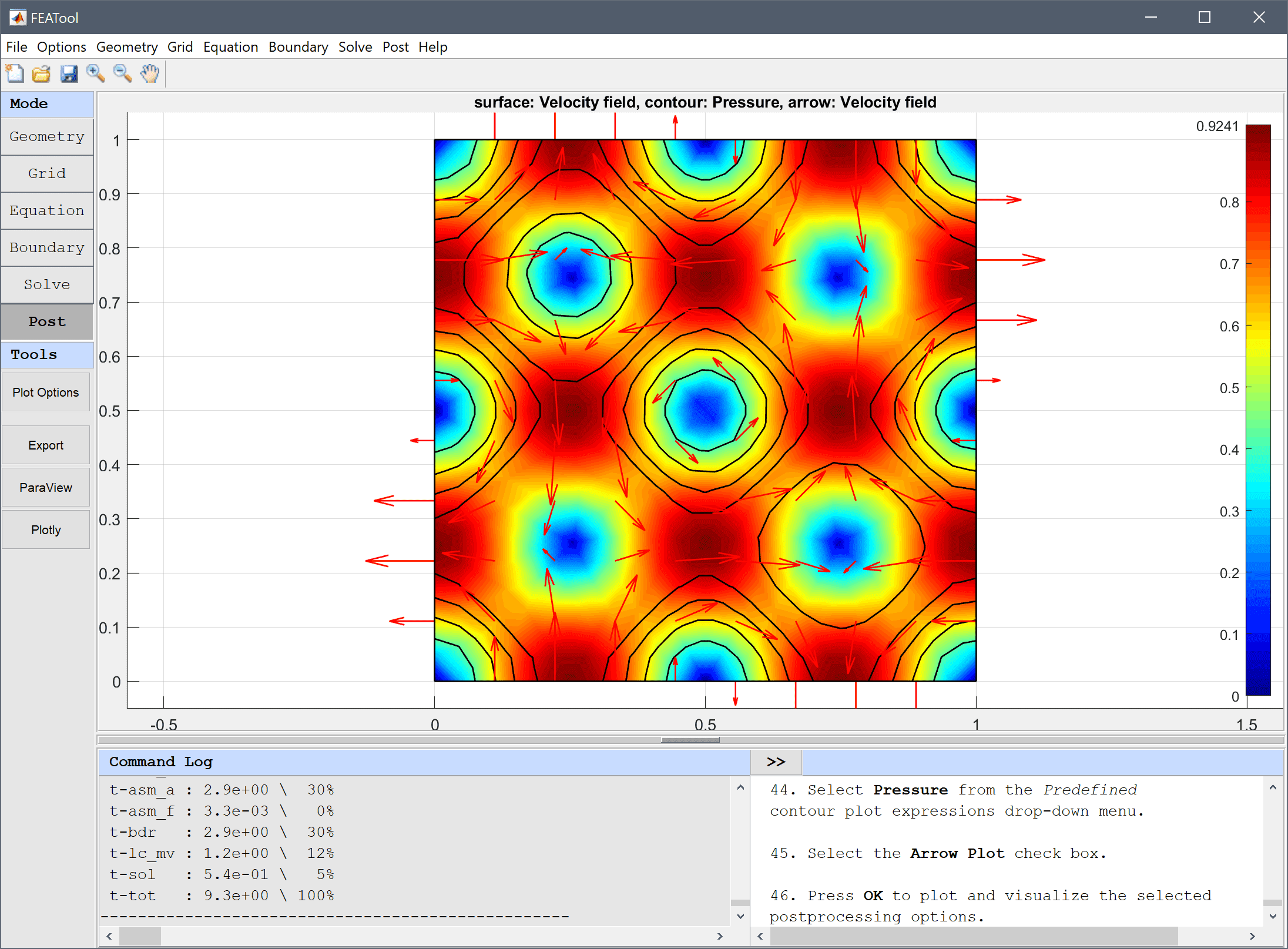
This example studies the time dependent decay from introducing standing vortices in a periodic domain. Due to the even spacing and counter rotation, the vortices will stay in place and simply loose intensity with time, and eventually the flow will return to a perfectly steady state. This is in fact one of the few model problems with and analytical solution to the non-linear incompressible Navier-Stokes equations
\[ \begin{array}{l} u = -cos(kx) sin(ky) e^{-2\nu k^2t} \\\\ v = sin(kx) cos(ky) e^{-2\nu k^2 t} \\\\ p = -\frac{1}{4}(cos(2kx)+cos(2ky)) e^{-4\nu k^2 t} \end{array} \]
The two-dimensional flow problem is solved for a unit square with k = 2π and the exact solution as boundary and initial conditions.
This model is available as an automated tutorial by selecting Model Examples and Tutorials… > Fluid Dynamics > Vortex Flow from the File menu, and also as the MATLAB simulation m-script example ex_navierstokes5. Step-by-step tutorial instructions to set up and run this model are linked below.