Fluid flows with swirl effects can occur in rotationally symmetric geometries where the azimuthal or angular velocity component is non-zero. In this case one must solve the fully three-dimensional Navier-Stokes equations. However, due to the assumption that azimuthal variations can be neglected, it is still sufficient to limit the simulations to axisymmetric 2D domains, thus saving significant amounts of computational time and effort.
The following examples describe how to set up and model axisymmetric systems with swirl effects in FEATool Multiphysics, and illustrate the modeling process with a selection of fluid dynamics and swirl flow examples.

Taylor-Couette Swirl Flow using the GUI
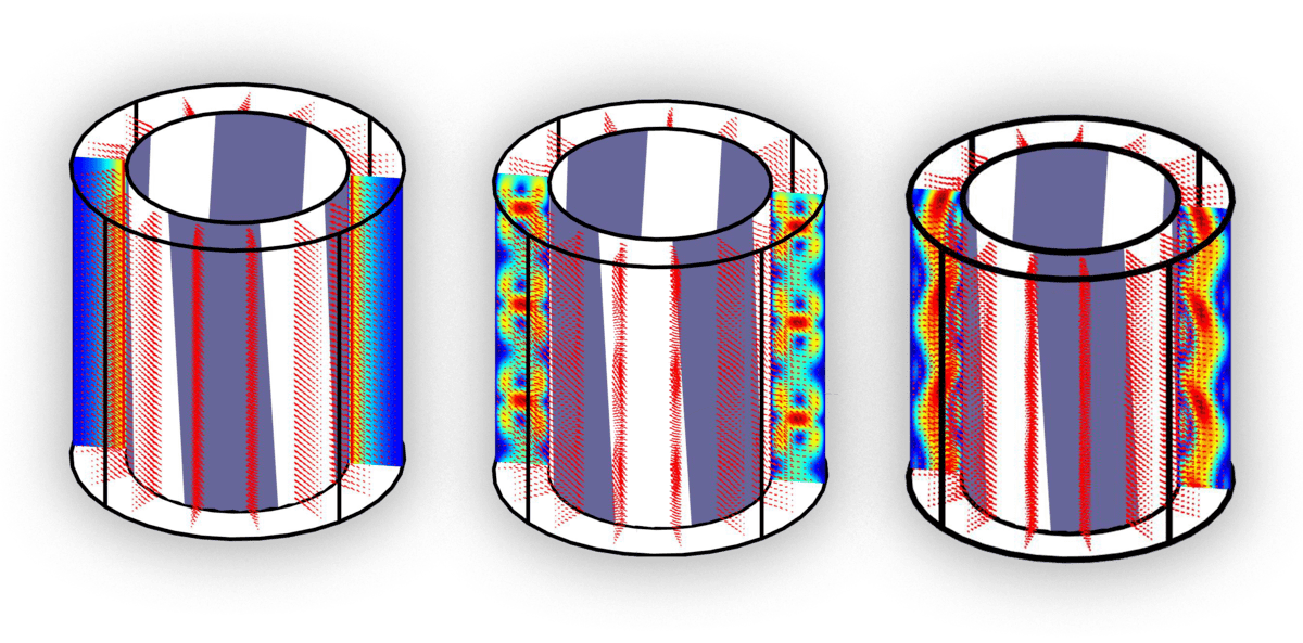
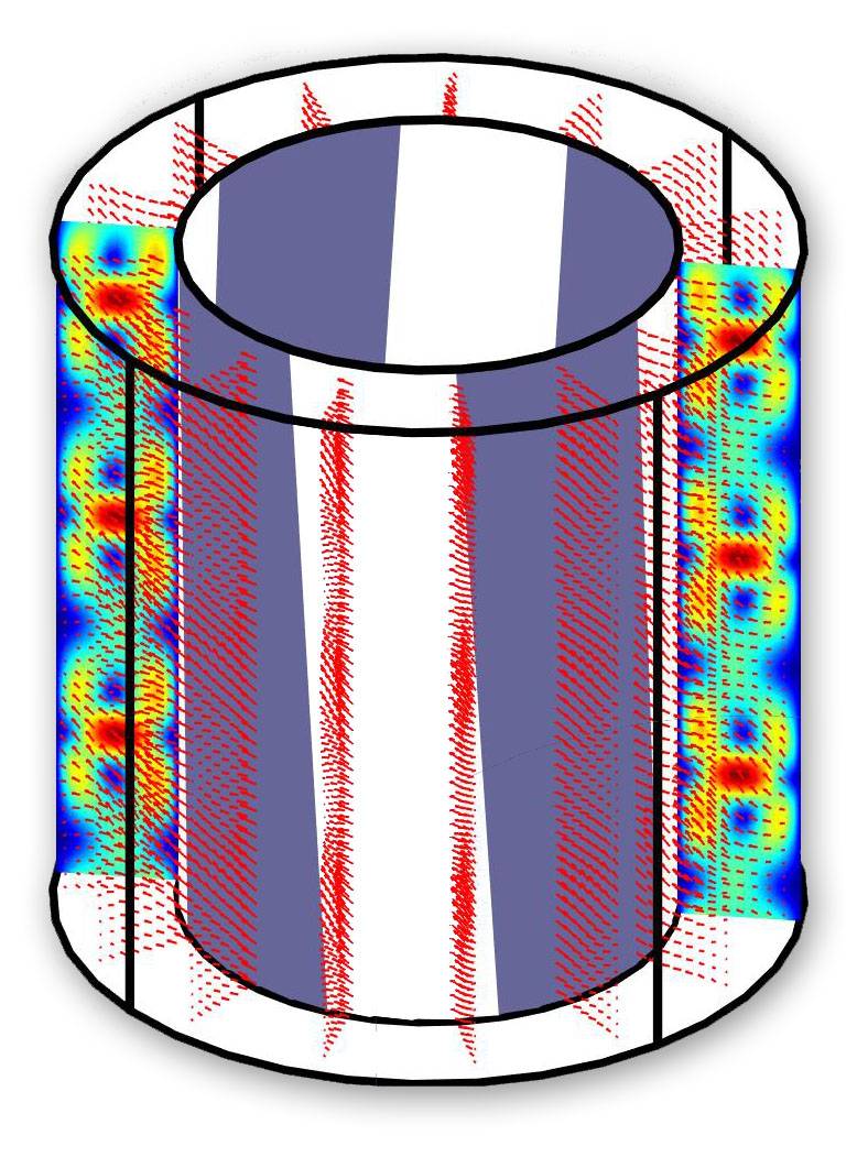
This example models axisymmetric flow between two concentric cylinders where the inner cylinder is rotating. This leads to swirl effects and so called Taylor-Couette flow with periodic and in-plane vortices.
The model is available as an automated tutorial by selecting Model Examples and Tutorials… > Fluid Dynamics > Taylor-Couette Swirling Flow from the File menu. Or alternatively, follow the linked step-by-step instructions.
Implementing Swirl Flow as Custom PDE Equations
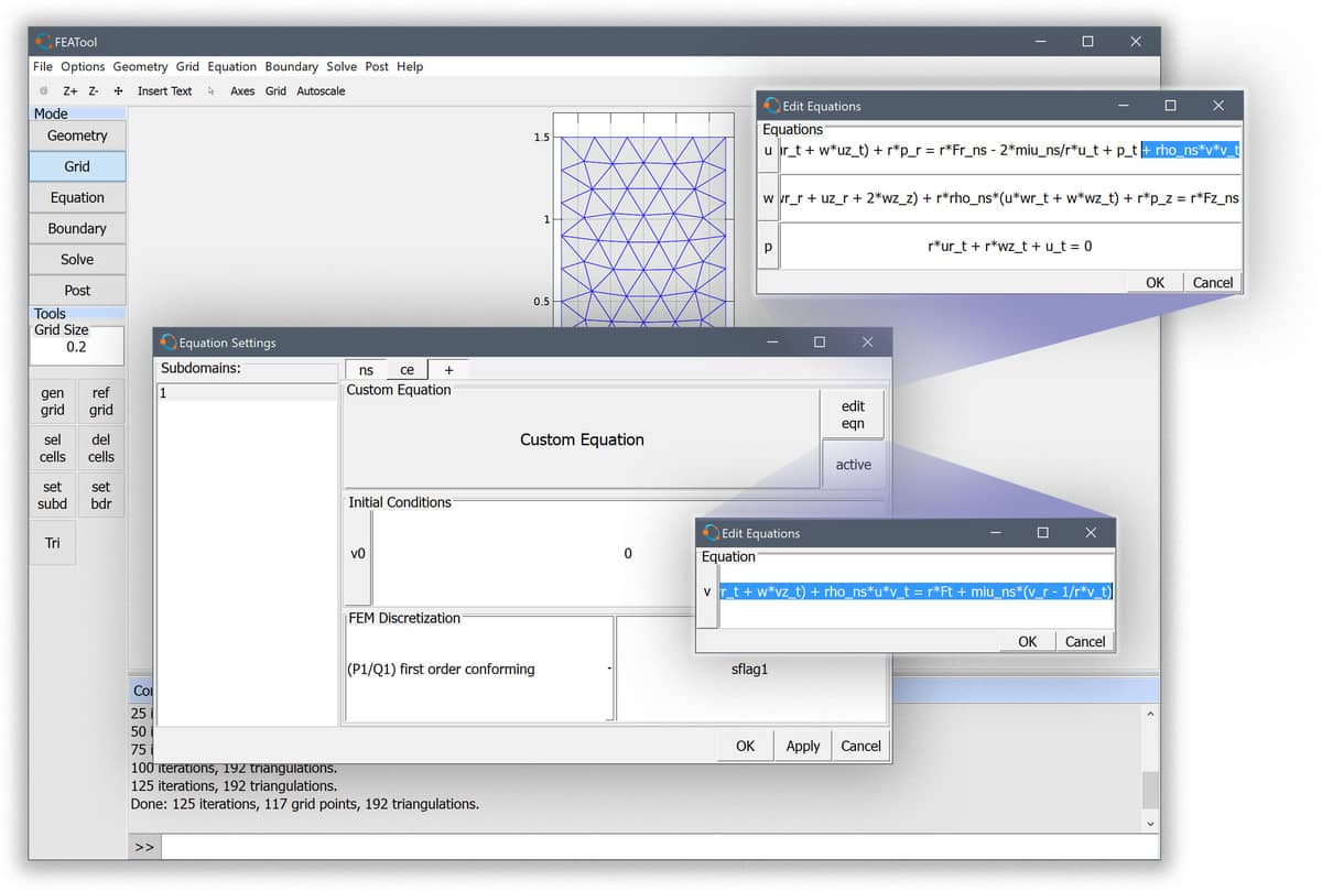
To model swirling flows with the FEATool GUI one can also use the axisymmetric Navier-Stokes physics mode and modify it. The u momentum equation in the radial direction must be extended with the non-linear source term ρv2, which can be done using the Edit Equation functionality in the Subdomain Settings dialog box.
Moreover, an additional equation for the radial velocity component must also be added. This can be achieved by adding a Custom Equation multiphysics mode with dependent variable named v, and corresponding momentum equation expression defined as
r*rho_ns*v' - r*miu_ns*(vr_r + vz_z) + ...
   miu_ns*v_r + r*rho_ns*(u*vr_t + w*vz_t) + rho_ns*u*v_t = ...
   r*Ft + miu_ns*(v_r - 1/r*v_t)
Even though the dependent variables here are split between two different physics modes the solver will automatically solve them as a fully coupled system.

In this implementation approach it is necessary to manually set the boundary condition for v separately, since swirl boundary conditions are not predefined. Moreover, as the predefined axisymmetric Navier-Stokes postprocessing expressions, such as velocity magnitude, do not include the v component, one has to re-define these manually as custom equation expressions if desired.
Swirl Flow using the MATLAB CLI
With FEATool Multiphysics one can also conveniently program and script the models on the MATLAB command line interfaces (CLI). The following example sets up a model for flow between two cylinders where the inner one is rotating and the outer is stationary. The first step is to define the model parameters, geometry, and grid
% Problem definition.
rho   = 1.0;   % Density.
miu   = 1.0;   % Molecular viscosity.
omega = 5.0;   % Angular velocity.
ri    = 0.5;   % Inner radius.
ro    = 1.5;   % Outer radius.
h     = 3.0;   % Height of cylinder.

% Geometry and grid generation.
fea.sdim = {'r' 'z'};
fea.geom.objects = { gobj_rectangle(ri,ro,-h/2,h/2) };
fea.grid = gridgen( fea, 'hmax', (ro-ri)/6 );
Next the, custom governing equations are defined, here directly without using any predefined physics modes
% Equation definition.
fea.dvar = { 'u', 'v', 'w', 'p' };
fea.sfun = [ repmat( {'sflag2'}, 1, 3 ) {'sflag1'} ];
c_eqn    = { 'r*rho*u'' - r*miu*(2*ur_r + uz_z  +   wr_z) + r*rho*(u*ur_t + w*uz_t) + r*p_r     = - 2*miu/r*u_t + p_t + rho*v*v_t';
             'r*rho*v'' - r*miu*(  vr_r + vz_z) + miu*v_r + r*rho*(u*vr_t + w*vz_t) + rho*u*v_t = miu*(v_r - 1/r*v_t)';
             'r*rho*w'' - r*miu*(  wr_r + uz_r  + 2*wz_z) + r*rho*(u*wr_t + w*wz_t) + r*p_z     = 0';
             'r*ur_t + r*wz_t + u_t = 0' };
fea.eqn = parseeqn( c_eqn, fea.dvar, fea.sdim );

fea.coef = { 'rho', rho ;
             'miu', miu };
For boundary conditions the inner wall is given a rotational velocity, while the outer is prescribed a no-slip wall, and the top and bottom zero normal flows
% Boundary conditions.
fea.bdr.d = { []  0 []  0 ;
              []  0 [] omega*ri ;
               0  0  0 [] ;
              [] [] [] [] };
fea.bdr.n = cell(size(fea.bdr.d));
The incompressible Navier-Stokes equations typically requires the pressure to be defined and fixed in at least one point. This is usually done with an outflow boundary, but since here there are no in- or out-flows, the pressure is simply fixed by setting the value of the top outer corner to zero
% Fix pressure at p([r,z]=[ro,h/2]) = 0.
[~,ix_p] = min( sqrt( (fea.grid.p(1,:)-ro).^2 + (fea.grid.p(2,:)-h/2).^2) );
fea.pnt = struct( 'type',  'constr', 'index', ix_p, 'dvar', 'p', 'expr', '0' );
To improve convergence, and compute a stationary solution faster, an analytic Newton Jacobian is defined (the non-linear Newton solver is activated when the jac solver argument is provided, otherwise standard fix-point iterations are used)
% Define analytical Newton Jacobian bilinear form.
jac.coef  = { 'r*rho*ur'       'rho*v' 'r*rho*uz' [] ;
              'r*rho*vr+rho*v' []      'r*rho*vz' [] ;
              'r*rho*wr'       []      'r*rho*wz' [] ;
              []               []      []         [] };
jac.form = cell(size(jac.coef));
[jac.form{~cellfun(@isempty,jac.coef)}] = deal([1;1]);
The complete problem can now be parsed and solved
% Parse and solve problem.
fea = parseprob( fea );
fea.sol.u = solvestat( fea, 'jac', jac );
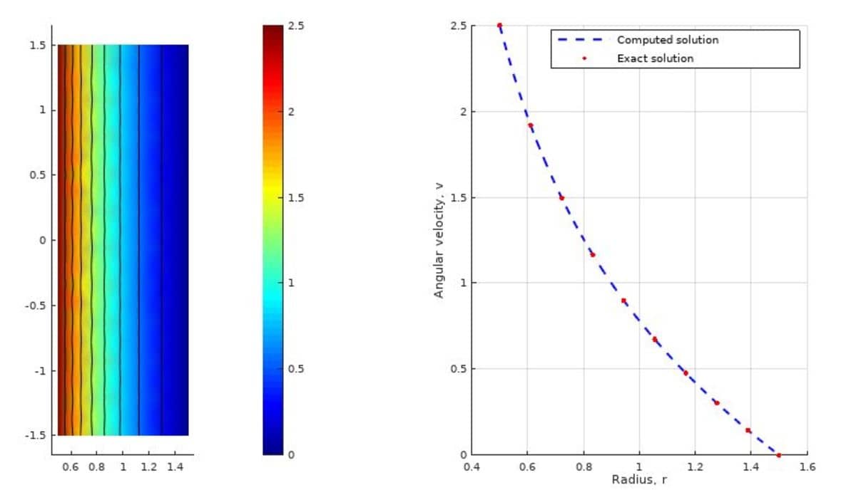
To verify the accuracy of the computed solution a comparison with an analytic solution (valid for small rotational velocities) is made
% Exact (analytical) solution.
a = - omega*ri^2 / (ro^2-ri^2);
b =   omega*ri^2*ro^2 / (ro^2-ri^2);
v_th_ex = @(r,a,b) a.*r + b./r;

% Postprocessing.
subplot(1,2,1)
postplot( fea, 'surfexpr', 'sqrt(u^2+v^2+w^2)', 'isoexpr', 'v' )

subplot(1,2,2)
hold on
grid on
r = linspace( ri, ro, 100 );
v_th = evalexpr( 'v', [r;zeros(1,length(r))], fea );
plot( r, v_th, 'b--' )
r = linspace( ri, ro, 10 );
plot( r, v_th_ex(r,a,b), 'r.' )
legend( 'Computed solution', 'Exact solution')
xlabel( 'Radius, r')
ylabel( 'Angular velocity, v')
From the figure below it is clear that very good agreement with the analytical solution has been achieved.

Transient Taylor-Couette Flow Simulation
A very interesting phenomena happens when the rotational velocity is increased, and after a certain point so called Taylor vortices appear. The flow is still laminar but exhibits lengthwise vortices. As the velocity is increased further they destabilize and start to travel in the axial direction. The video below show this behavior, in particular observe around t = 10 s when the stable Taylor vortices appear (at about Taylor number Ta = 1500 - 1700 which is in good agreement with theory), and t = 20 s when they start moving length wise.
The time-dependent Taylor-Couette flow script model is available from the FEATool models and examples directory as the ex_swirl_flow3 model m-script file (note that periodic boundary conditions are implemented with an external solve_hook function which is discussed in the periodic boundary condition tutorial.
