Parametric studies can be very useful tools to clearly see how a model or simulation will behave under varying conditions. The following post presents a parametric study of the 3D bracket deflection model introduced previously where both the geometry, in this case plate thickness, and also the applied load force is varied.
The first step in creating a parametric model is to save the model as an m-script model file. This can be done by selecting Save as M-Script Model from the File menu.
Open the file in your favorite editor. It is now possible to see exactly which steps and functions were used in creating the model. The first change to make is to add vectors of parameters at the top of the file
 thickness = [ 0.02 0.015 0.01 0.008 ];
 loads     = [ 1e4 2e4 1e5 1e6 ];
3. The second change is to replace the geometry and grid operations with the following code so that the thickness of the second block will be varied with the iteration counter _i_
     for i=1:length(thickness)

     % Geometry operations.
     fea.geom = struct;
     gobj = gobj_block( 0, 0.02, 0, 0.2, 0, 0.2, 'B1' );
     fea  = geom_add_gobj( fea, gobj );
     gobj = gobj_block( 0, 0.2, 0, 0.2, ...
                   0.1-thickness(i)/2, 0.1+thickness(i)/2, 'B1' );
     fea  = geom_add_gobj( fea, gobj );
     gobj = gobj_cylinder( [ 0.1, 0.1, 0.08 ], 0.08, 0.04,3,'C1');
     fea  = geom_add_gobj( fea, gobj );
     fea  = geom_apply_formula( fea, 'B1+B2-C1' );

     % Grid generation.
     fea.grid = gridgen( fea, 'hmax', thickness(i)/2 );
4. As second loop can now be introduced where the varying load is extracted and prescribed by using a constant variable. The equation settings can be kept from the saved model.
     for j=1:length(loads)

     % Constants and expressions.
     fea.expr = { 'load', loads(j) };

     % Equation settings.
     fea.phys.el.dvar = { 'u', 'v', 'w' };
     fea.phys.el.sfun = { 'sflag1', 'sflag1', 'sflag1' };
     fea.phys.el.eqn.coef = { 'nu_el', ', '', { '0.3' };
     ...
Two loops have now been set up around the model, the first creating a geometry with varying thickness, and the second will prescribe the varying load. Note that setting up the loops in this way allows reusing the grid in the inner loop and saving computational time.
When the grid changes the boundary numbering may also change. The static boundary condition prescription must therefore be replaced with one that identifies the correct boundaries. This can be achieved in the following way
 % Boundary conditions.
 n_bdr = max(fea.grid.b(3,:));
 ind_fixed = findbdr( fea, 'x<0.005' );
 ind_load  = findbdr( fea, 'x>0.19'  );
 fea.phys.el.bdr.sel = ones(1,n_bdr);

 % Define Homogeneous Neumann BC type.
 n_bdr  = max(fea.grid.b(3,:));
 bctype = num2cell( zeros(3,n_bdr) );

 % Set Dirichlet BCs for the fixed boundary.
 [bctype{:,ind_fixed}] = deal( 1 );
 fea.phys.el.bdr.coef{1,end-2} = bctype;

 % Define all zero BC coefficients.
 bccoef = num2cell( zeros(3,n_bdr) );

 % Apply negative z-load to outer edge.
 [bccoef{3,ind_load}] = deal( '-load' );

 % Store BC coefficient array.
 fea.phys.el.bdr.coef{1,end} = bccoef;
6. When the problem is fully specified we can call the solver, apply postprocessing to calculate the maximum stress, and close the loops
     % Solver call.
     fea = parsephys( fea );
     fea = parseprob( fea );
     fea.sol.u = solvestat( fea );

     % Postprocessing.
     s_vm = fea.phys.el.eqn.vars{1,2};
     vm_stress = evalexpr( s_vm, fea.grid.p, fea );
     max_vm_stress(i,j) = max(vm_stress);

     end,end
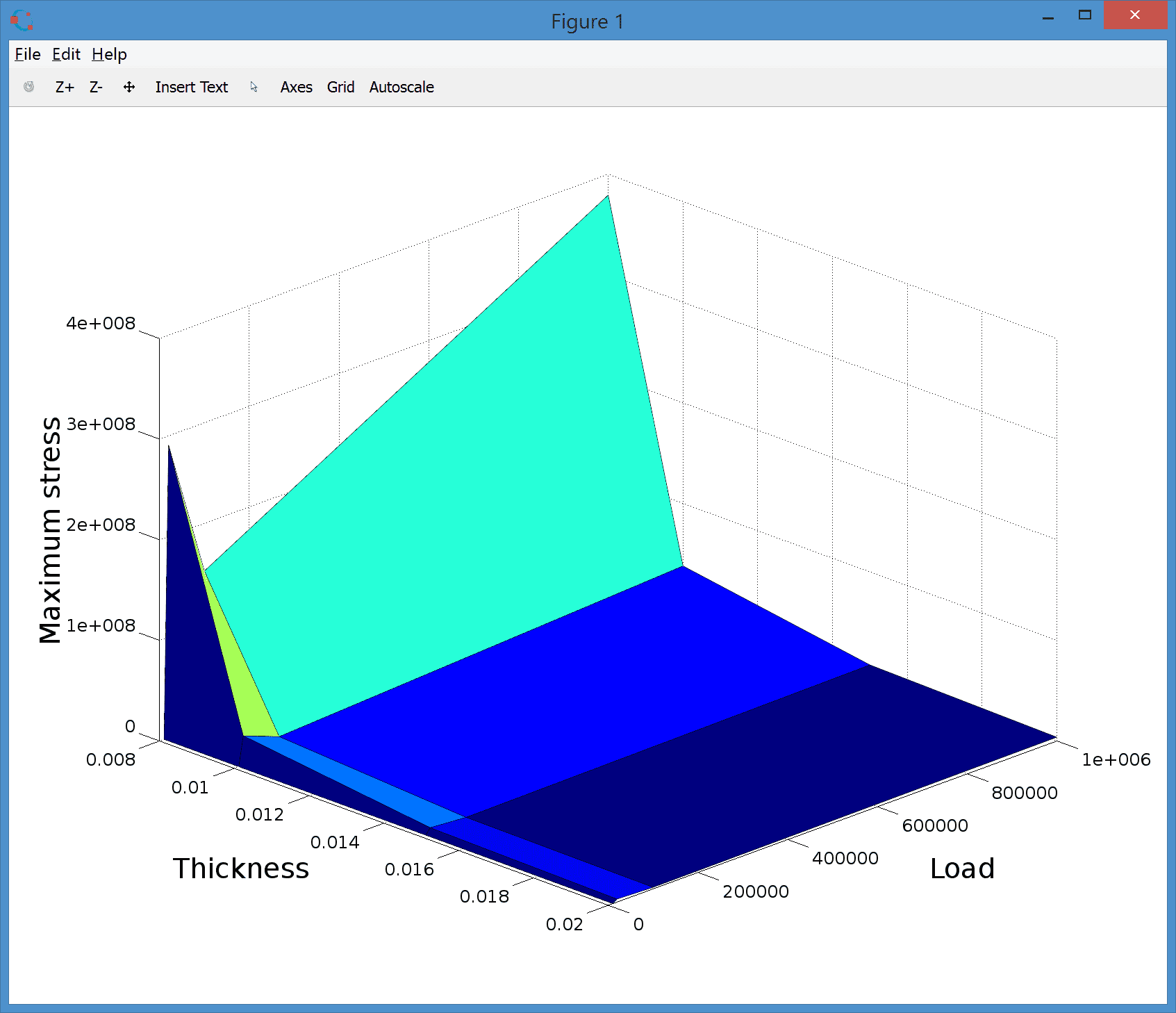
7. Finally visualize the all computed maximum stresses at once as
     % Visualization.
     [t,l] = meshgrid(thickness,loads);
     surf( t, l, max_vm_stress, log(max_vm_stress) )
     xlabel( 'Thickness' )
     ylabel( 'Load' )
     zlabel( 'Maximum stress' )
     view( 45, 30 )