FEATool has been designed with flexibility and user customization in mind allowing for solving custom equations, calling external solvers, grid generators, and post processing tools, and allowing for both MATLAB m-script as well as GUI based modeling. This post shows how to easily define custom finite element shape functions (also called basis functions or ansatz functions) which can be of interest for researchers, teachers, and advanced FEM users.
In the following a fifth order Lagrangian 1D FEM shape function will be defined, allowing for very accurate polynomial solutions with few grid cells. The first step is to create the function file, in this case we will call it sf_line_P5.m. The first header line of a shape function file should look like the following
function [ vBase, nLDof, xLDof, sfun ] = sf_line_P5( i_eval, n_sdim, n_vert, i_dof, xi, aInvJac, vBase )
The input arguments are; i_eval the evaluation type flag, n_sdim number of space dimensions, n_vert the number of vertices per grid cell, i_dof the shape or basis function to evaluate, xi local cell evaluation coordinates, aInvJac inverse of the transformation Jacobian, and vBase the output vector.
The output nLDof specifies the number of shape functions (degrees of freedom/unknowns) associated with grid cell vertices, edges (in 2D and 3D), faces (in 3D), and cell interiors. In this case we have two shape functions for each of the line end points and four equally spaced internal ones, thus nLDof here is
nLDof = [ 2 0 0 4 ];
xLDof specifies the location or position of each shape
function/dof in local cell coordinates. Barycentric (area/volume)
coordinates are used for lines and simplex cell shapes (triangles and
tetrahedra), and -1 … 1 local reference coordinates for
quadrilateral and hexahedral cells. It is important to number and
order the shape functions and corresponding coordinates associated
with vertices first, followed by edges, faces, and cell lastly
interiors (in counterclockwise direction in 2D and 3D). For the one
dimensional $P_5$ element we thus have the following coordinates
[ 1 0 4/5 3/5 2/5 1/5 ] and due to using barycentric
coordinates the second coordinate row is simply 1 minus the first
one ($\xi_2 = 1 - \xi_1$), we therefore have
xLDof = [ 1 0 4/5 3/5 2/5 1/5 ;
          0 1 1/5 2/5 3/5 4/5 ];
sfun simply returns the function name (for quick and easy function access during nested calls)
sfun = 'sf_line_P5';
The i_eval input flag is used to determine if either function value evaluations should be computed (i_eval = 1), or x, y, or z derivatives (i_eval = 2, 3, or 4, respectively). Furthermore, i_dof specifies for which of the basis functions evaluation should be performed, and vBase is the final output vector. We can now program the rest of the shape function evaluation definitions for the $P_5$ line element. (MATLAB source code for other shape function definitions can be found in the featool/ellib folder.)
switch i_eval

  case 1   % Function values.

    switch i_dof   % Shape/basis function.
      case 1
        vBase = (625*xi(1)^5)/24 - (625*xi(1)^4)/12 + (875*xi(1)^3)/24 - (125*xi(1)^2)/12 + xi(1);
      case 2
        vBase = - (625*xi(1)^5)/24 + (625*xi(1)^4)/8 - (2125*xi(1)^3)/24 + (375*xi(1)^2)/8 - (137*xi(1))/12 + 1;
      case 3
        vBase = - (3125*xi(1)^5)/24 + (6875*xi(1)^4)/24 - (5125*xi(1)^3)/24 + (1525*xi(1)^2)/24 - (25*xi(1))/4;
      case 4
        vBase = (3125*xi(1)^5)/12 - 625*xi(1)^4 + (6125*xi(1)^3)/12 - (325*xi(1)^2)/2 + (50*xi(1))/3;
      case 5
        vBase = - (3125*xi(1)^5)/12 + (8125*xi(1)^4)/12 - (7375*xi(1)^3)/12 + (2675*xi(1)^2)/12 - 25*xi(1);
      case 6
        vBase = (3125*xi(1)^5)/24 - (4375*xi(1)^4)/12 + (8875*xi(1)^3)/24 - (1925*xi(1)^2)/12 + 25*xi(1);
    end

  case 2   % x-derivative values.

    switch i_dof   % Shape/basis function.
      case 1
        dNdxi1 = (3125*xi(1)^4)/24 - (625*xi(1)^3)/3 + (875*xi(1)^2)/8 - (125*xi(1))/6 + 1;
      case 2
        dNdxi1 = - (3125*xi(1)^4)/24 + (625*xi(1)^3)/2 - (2125*xi(1)^2)/8 + (375*xi(1))/4 - 137/12;
      case 3
        dNdxi1 = - (15625*xi(1)^4)/24 + (6875*xi(1)^3)/6 - (5125*xi(1)^2)/8 + (1525*xi(1))/12 - 25/4;
      case 4
        dNdxi1 = (15625*xi(1)^4)/12 - 2500*xi(1)^3 + (6125*xi(1)^2)/4 - 325*xi(1) + 50/3;
      case 5
        dNdxi1 = - (15625*xi(1)^4)/12 + (8125*xi(1)^3)/3 - (7375*xi(1)^2)/4 + (2675*xi(1))/6 - 25;
      case 6
        dNdxi1 = (15625*xi(1)^4)/24 - (4375*xi(1)^3)/3 + (8875*xi(1)^2)/8 - (1925*xi(1))/6 + 25;
    end

    vBase = aInvJac(:,1) * dNdxi1;

  otherwise
    vBase = 0;

end

% end function sf_line_P5
Note that working in one dimension here it is enough to use one of the barycentric coordinates in the basis function definitions, here xi(1) (since xi(2) = 1 - xi(1)). Also, the derivative in local coordinates dNdxi1 is converted to global coordinates dNdx by multiplication with the inverse of the grid cell transformation Jacobian aInvJac, which in 1D is equal to the inverted grid cell width.
In contrast to typical FEM codes where matrix assembly is performed first in a loop over grid cells and then a loop over quadrature points, the FEATool FEM assembly operations are vectorized and performed in a single loop over quadrature points for groups of several cells at the same time. Thus the output vBase is a row vector with the same number of rows as aInvJac. However, as is done here for i_eval = 1 it is usually sufficient to compute and return a scalar value when the shape function evaluation for a quadrature point xi is independent of the real grid cell shapes. The assembly caller function then assigns this scalar value to the corresponding output vector entries.
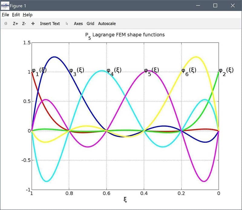
To plot and visualize the defined shape functions we can use the script below
xi = linspace( 0, 1, 100 );
grid on, hold on
colours = {' r' 'g' 'b' 'c' 'm' 'y' };
for i_dof=1:6
  for j=1:numel(xi)
    [phi(i_dof,j),~,xLDof] = sf_line_P5( 1, 1, 2, i_dof, xi(j) );
  end
  plot( xi, phi(i_dof,:), colours{i_dof} )
  text( xLDof(1,i_dof), 1, ['\phi_',num2str(i_dof),'(\xi)'] )
  xlabel( '\xi' )
end
title( 'P_5 Lagrange FEM shape functions' )
set( gca, 'xdir', 'reverse' )

We can also confirm that the sum of the basis functions is equal to unity over the defined span 0…1
phi_sum = all( abs( sum(phi,1) - 1 ) < sqrt(eps) )
To test the new shape function we set up and solve a simple Poisson equation with a polynomial source term and exact analytical solution
\[ \left\{\begin{aligned} \Delta u &= 140x^3 - 108x^2 + 18x - 4 \\\ u(x) &= -7x^5 + 9x^4 - 3x^3 + 2x^2 - 2x \end{aligned}\right. \]
fea.sdim = { 'x' };
fea.grid = linegrid( 1 );
fea.dvar = { 'u' };
fea.sfun = { 'sf_line_P5' };

% System matrix.
fea.eqn.a.form = { [2;2] };
fea.eqn.a.coef = { 1 };

% Source term.
fea.eqn.f.form = { 1 };
fea.eqn.f.coef = { '140*x^3 - 108*x^2 + 18*x - 4' };

% Boundary conditions.
fea.bdr.d = { 0  -1 };
fea.bdr.n = { [] [] };

% Solution.
fea.sol.u = solvestat( fea, 'icub', 5 );
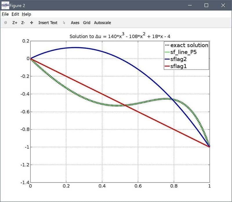
In this case we have solved the equation on a single grid cell. We can plot the solution and compare with the exact analytical one, and also with linear and quadratic shape functions. (Note that the solver parameter icub has been increased to 5 from the default 2 so that the numerical integration can accurately integrate the 5th order polynomials).
% Postprocessing.
x    = linspace( 0, 1, 100 );
uref = evalexpr( '-7*x^5 + 9*x^4 - 3*x^3 + 2*x^2 - 2*x', x, parseprob(fea) );
u5   = evalexpr( 'u', x, parseprob(fea) );

fea.sfun  = { 'sflag2' };
fea.sol.u = solvestat( fea );
u2 = evalexpr( 'u', x, parseprob(fea) );

fea.sfun  = { 'sflag1' };
fea.sol.u = solvestat( fea );
u1 = evalexpr( 'u', x, parseprob(fea) );

grid on, hold on
plot( x, uref, 'k--', 'linewidth', 2 )
plot( x, u5,   'g-'  )
plot( x, u2,   'b-'  )
plot( x, u1,   'r-'  )
hl = legend( 'exact solution', 'sf_line_P5', 'sflag2', 'sflag1' );
title( 'Solution to \Deltau = 140*x^3 - 108*x^2 + 18*x - 4' )

We can see that the $P_5$ shape function gives the exact solution with just a single grid cell while the $P_1$ and $P_2$ shape functions require more cells to achieve a better approximation.
It is also possible to use custom shape functions in the FEATool GUI by entering the corresponding shape function name in the FEM Discretization field of the Equation Settings dialog box (and also increasing the Numerical integration rule order in the Solver Settings dialog box).
