Coupled Multiphysics Modeling of Resistive Heating in a Tungsten Filament

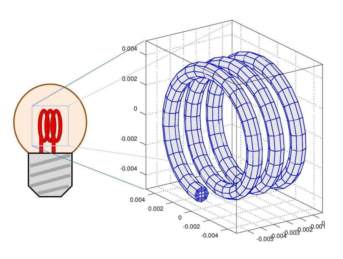
The following tutorial discusses multiphysics modeling of resistive Joule heating simulated with the FEATool Multiphysics MATLAB FEM toolbox. In the model the resulting current from an applied electric potential will heat a thin spiral shaped Tungsten wire, such as can be found in incandescent light bulbs. After the start up phase the filament reaches an equilibrium temperature where the internal heat generation is balanced by radiative heat loss through the boundaries. Although the model could quite easily be implemented in the FEATool GUI, since it features a one way multiphysics coupling it will be shown how the dependent variables and equations can be decoupled and implemented as a MATLAB m-script file to save computational time.

Model parameters and constants

The first modeling step is to define constants for the equation coefficients and boundary conditions. It is assumed the material of the filament is Tungsten and is held at 20 ℃ at its connecting points in the socket, and is also subject to radiative heat loss with an ambient temperature of 80 ℃. An electric potential of 0.2 V is applied across the wire resulting in temperature rise due to the source term Q. Here, we label this term with the coefficient string qfunction which FEATool will attempt to parse as a general string expression. (Valid equation, boundary, and postprocessing string expressions may consist of combinations of numerical values, dependent variables and derivatives, here V and Vx etc., space coordinates x, y, and z, built-in constants and functions such as pi and sin, and custom functions). Here we will use the fact that as a last resort FEATool will try to parse and evaluate qfunction as a custom user-defined MATLAB m-function the construction of which will be discussed later.

V0    = 0.2;          % Potential difference [V].
sigma = 1/52.8e-9;    % Electrical conductivity [1/Ohm/m].

rho   = 19.25e3;      % Density [kg/m3].
cp    = 133.9776;     % Specific heat capacity [J/kg/K].
k     = 173;          % Thermal conductivity [W/m/K].
Q     = 'qfunction';  % Resistive heating source term function.

C     = 5.670367e-8;  % Stefan-Bolzmann radiation constant.
T0    = 20 + 273.15;  % Initial temperature [K].
Tamb  = 80 + 273.15;  % Mean ambient temperature [K].

Grid generation

Since the geometry in this case is quite simple we can omit it and directly proceed to manually create the grid through using the grid primitive functions (fea.geom fields are only used by the unstructured grid generation function gridgen). The computational grid is thus here created by taking a circle circgrid, extruding, and revolving it to create the filament spiral gridrevolve.

% Geometry dimensions in [m].
r_wire   = 0.0005;   % Wire radius.
l_spiral = 0.005;    % Length of spiral.
r_spiral = 0.004;    % Outer radius of spiral.

fea.sdim = { 'x' 'y' 'z' };
fea.grid = gridrotate( gridrevolve( ...
             circgrid( 2, 3, r_wire ), ...
                       80, l_spiral, 3, r_spiral ), ...
                        -pi/2, 2 );

The resulting grid and boundaries can be visualized with the plotgrid(fea) and plotbdr(fea) commands, respectively.

Electrostatics

The model is quasi-static in the sense that the electric potential solution is static while the overall heat transfer process is examined as a function of time. Although we could solve this as a monolithically coupled problem (solving for T and V simultaneously together), the electric potential problem is assumed to be independent of the temperature (the electrical conductivity $\sigma$ is constant) and can thus be solved separately as a steady state problem by itself, that is

\[ \nabla\cdot(\sigma\nabla V) = 0 \]

with insulation boundary conditions, $\mathbf{n}\cdot(\sigma\nabla V)=0$, everywhere except for the two ends where the potential difference V0 is applied. In the MATLAB m-script of language used by FEATool this looks like the following

% Set up and solve electrostatics problem.
feaV = addphys( fea, @conductivemediadc );

feaV.phys.dc.eqn.coef{2,end} = {sigma};   % Electrical conductivity.

feaV.phys.dc.bdr.sel([1 98])    = 1;
feaV.phys.dc.bdr.coef{1,end}{1} = V0;     % Potential difference.

feaV = parsephys( feaV );
feaV = parseprob( feaV );
feaV.sol.u  = solvestat( feaV );

Note that here an alternative help variable for the FEM struct belonging to the electric potential has been used, feaV.

Heat transfer

The heat transfer problem for the temperature field is governed by the heat equation PDE

\[ \rho c_p\frac{\partial T}{\partial t} - \nabla\cdot (k\nabla T) = Q \]

where here the electric potential is also the source of heat generation with the term $Q = \sigma|\nabla V|^2$. Thus this equation features a non-linear one-way multiphysics coupling, V coupled to the temperature T. As for interaction with the surroundings the temperature is fixed at T = T0 at both ends while radiation flux boundary conditions $\mathbf{n}\cdot(k\nabla T)=C(T_{amb}^4-T^4)$ are applied everywhere else. The following code sets up this heat transfer problem

% Set up heat transfer problem.
fea = addphys( fea, @heattransfer );

fea.phys.ht.eqn.coef{1,end} = {rho};   % Density.
fea.phys.ht.eqn.coef{2,end} = {cp};    % Heat capacity.
fea.phys.ht.eqn.coef{3,end} = {k};     % Thermal conductivity.

% Use generalized heat flux boundary condition (4) for all boundaries
% except at the ends where the temperature T0 is prescribed(1).
fea.phys.ht.bdr.sel([2:97]) = deal(4);
[fea.phys.ht.bdr.coef{4,end}{2:97}] = deal({0 0 0 C Tamb});

fea.phys.ht.bdr.sel([1 98]) = deal(1);
fea.phys.ht.bdr.coef{1,end}{ 1} = T0;
fea.phys.ht.bdr.coef{1,end}{98} = T0;

% Specify heat source term - qfunction.
fea.phys.ht.eqn.coef{7,end} = {'qfunction'};
% Add sigma and electric potential solution used by qfunction.
fea.expr = { 's_sigma' '' '' sigma ;
             'u_V'     '' '' feaV.so.u };

Custom external source term function

We cannot solve the temperature problem yet since we have not defined the heat source term qfunction. We do this in a separate MATLAB m-file with the same name as the equation coefficient itself, that is qfunction.m. Although the following code for qfunction might look intimidating, all it does is to essentially take the solution for V stored in fea.expr and computes the heat source term as sigma*(Vx^2+Vy^2+Vz^2). Although we could easily solve the fully monolithically coupled problem with the FEATool GUI, we would then have to solve a much larger coupled system in each time step. This decoupled approach we save both time and memory at the cost of having to use a custom function.

function [ Q ] = qfunction()
% Build up a source term expression from the precomputed solution
% vector stored in prob.expr{ u_V }. Expected to be called from evalexpr0.

% Workaround to get input variable string names from evalexpr0.
persistent inputname0
if( isempty(inputname0) )
  ds    = dbstack;
  fid   = fopen( which(ds(2).file), 'r' );
  sline = fgetl( fid );
  sline = sline( find( sline== '(', 1 )+1:find( sline== ')', 1 )-1 );
  inputname0 = regexp( sline(~isspace(sline)), ',', 'split' );
  fclose( fid );
end

% Extract variable from the calling function, evalexpr0.
xi    = evalin( 'caller', inputname0{2} );
ind_s = evalin( 'caller', inputname0{3} );
ind_c = evalin( 'caller', inputname0{4} );
prob  = evalin( 'caller', inputname0{6} );
aJac  = evalin( 'caller', inputname0{7} );

n_sdim = size( prob.grid.p, 1 );
n_vert = size( prob.grid.c, 1 );

i_dvar = 1;   % Assume same dep. var. fem basis function for u_V as for i_dvar=1.
[~,~,~,sfun] = evalsfun( prob.sfun{i_dvar}, 0, n_sdim, n_vert );   % Get shape function root string.
if( isempty(aJac) )   % Calculate Jacobian if required.
  store_aJTmp = strcmpi(sfun(end-1:end),'H3') && ( (n_sdim==2 && n_vert==4) || (n_sdim==3 && n_vert==8) );
  [~,aJac] = tfjac( 1, prob.grid.p, prob.grid.c(:,ind_c), [], xi, aJac, store_aJTmp );
end

u_V = prob.expr{ find(strcmp(prob.expr,'u_V')), end };   % V solution vector.

% Evaluate derivatives of V (1=function value, 2=x-derivative, 3=y-derivative, 4=z-derivative).
Vx  = evaldvar( sfun, 2, n_sdim, n_vert, xi, aJac, prob.eqn.dofm{i_dvar}(:,ind_c), u_V );
Vy  = evaldvar( sfun, 3, n_sdim, n_vert, xi, aJac, prob.eqn.dofm{i_dvar}(:,ind_c), u_V );
Vz  = evaldvar( sfun, 4, n_sdim, n_vert, xi, aJac, prob.eqn.dofm{i_dvar}(:,ind_c), u_V );

% Value or expression for sigma.
s_sigma = prob.expr{ find(strcmp(prob.expr,'s_sigma')), end };

% Calculate final expression and return values.
Q = evalexpr0( s_sigma, xi, ind_s, ind_c, [], prob, aJac ).*( Vx.^2 + Vy.^2 + Vz.^2 );

Solution and postprocessing

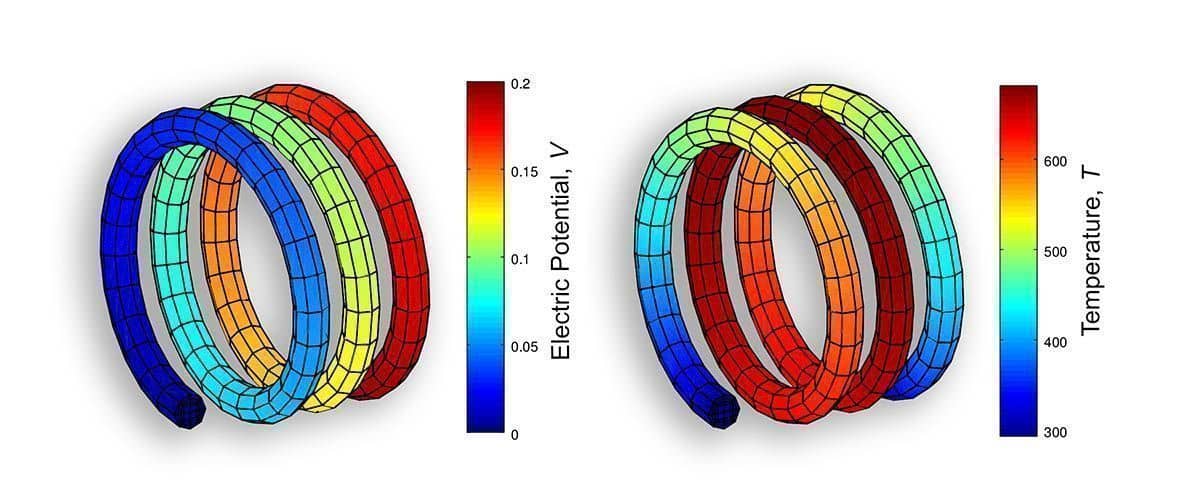
Finally we can solve the time-dependent heat transfer problem and plot the solutions keeping in mind that the electric potential is stored in the feaV FEM struct and temperature separately in fea.

fea = parsephys( fea );
fea = parseprob( fea );
fea.sol.u = solvetime( fea, 'init', {T0}, 'tstep', 1, 'tmax', 20 );

figure
subplot(1,2,1)
postplot( feaV, 'surfexpr', 'V' )
subplot(1,2,2)
postplot( fea, 'surfexpr', 'T' )

After the solver has finished we can see that the maximum reached temperature is about 700 K. The temporal evolution of the temperature field can also be seen in the video linked below. Technically, we could continue our study by also examining the heat induced stresses and strains, coupling the temperature to the linear elasticity physics mode. However since for this particular application the failure point is likely to be due to temperature, which is far lower than the melting temperature of Tungsten, it is safe to assume that we do not need to examine the stresses.

The described resistive heating MATLAB model m-file is available from the FEATool examples directory as ex_resistive_heating1.