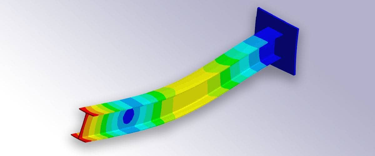
This post will discuss how to implement and model elastic deformations of simple beams with FEATool Multiphysics. Although also available as a pre-defined physics mode and GUI option, beams and truss structures can also be implemented and accurately simulated with slight extension of the available FEM MATLAB functions and subroutines. The following modeling example will be limited to small deformations according to Euler-Bernoulli beam theory.
Static deformation
For modeling the static vertical deflections, v(x) of a horizontal beam the following fourth order equation applies
\[ -\frac{\partial^2 }{\partial x^2}(EI(x)\frac{\partial^2 v}{\partial x^2}) = q(x) \]
where E is the modulus of elasticity, I(x) cross-section moment of inertia, and q(x) any applied volume load or force.
Due to the partial integration in the finite element weak formulation it is sufficient with basis functions with non-vanishing 2nd derivatives. Traditionally FEM beam simulations employ the 3rd order Hermite finite element. Although FEATool currently does not include support for evaluating 2nd order derivatives, the open design of the source code makes this easy to support simply by including the following i_eval case in the sf_line_H3 m-file definition (for more regarding custom finite element shape functions in MATLAB script code see the previous post on implementing user defined FEM basis functions
function [ vBase, nLDof, xLDof, sfun ] = ...
           sf_line_H3( i_eval, n_sdim, n_vert, i_dof, xi, aInvJac, vBase )
...

case 22   % Evaluation of second derivatives.

  switch i_dof   % Basis function derivative to evaluate.
    case 1
      dNdxi1 =  6*(2*xi(1)-1) ./ aInvJac(:,3);
      dNdxi2 =  0;
    case 2
      dNdxi1 =  0;
      dNdxi2 = -6*(2*xi(2)-1) ./ aInvJac(:,3);
    case 3
      dNdxi1 =  6*xi(1) - 2;
      dNdxi2 =  0;
    case 4
      dNdxi1 =  0;
      dNdxi2 =  6*xi(2) - 2;
  end

  vBase = aInvJac(:,1) .* dNdxi1 + aInvJac(:,2) .* dNdxi2;

  ....
In addition to the standard i_eval = 1 function value, and 2/3/4 x/y/z-derivative evaluations, we have created the new case 22 for the x2-derivative.
To define the simulation model we first create a finite element analysis fea struct with a line grid spanning from 0 to L with nx cells
% Grid generation.
fea.sdim = {'x'};   % Space dimension coordinate name.
fea.grid = linegrid( nx, 0, L );
We define the PDE equation for the y-displacement v
% Problem and equation definitions.
fea.dvar{1} = 'v';            % Dependent variable name.
fea.sfun{1} = 'sf_line_H3';   % FEM shape function for v.
eqn_v       = '-E*I*vx_x = q';
Note here that this equation specifies vx_x for the bilinear form, not vxx_xx which one would like. This is due to the fact that the FEATool equation parser not yet supports 2nd order derivatives, thus vx_x is used as a temporary placeholder. Furthermore, we also add a help equation for the rotation $\theta$
fea.dvar{1} = 'th';           % Help variable name.
fea.sfun{1} = 'sflag2';
eqn_th      = 'th_t - vx_t = 0';
This help equation is not essential and does not influence the solution since it simply is an algebraic expression for $\theta = \frac{\partial v}{\partial x}$. We will however use the th variable in postprocessing, or more accurately thx = $\frac{\partial \theta}{\partial x}$, which is equivalent to the 2nd derivative of v used in calculating the bending moment.
Having specified the equations we can call the FEATool equation parser which processes the string equations into the weak finite element definitions into the fea.eqn fields
fea.eqn  = parseeqn( { eqn_v, eqn_th }, fea.dvar, fea.sdim );

fea.eqn.a.form{1} = [22;22];
Note here that we manually substitute the first weak a bilinear form
component from [2;2] (due to vx_x) to
[22;22] which will correspond to the sought term
vxx_xx. What this simply means in practical terms is that in the
FEM system matrix assembly step an i_eval flag of 22 will be
passed to the FEM trial and test shape function routine instead of the
usual 2.
Boundary conditions also need to be prescribed, in this case the assumption is the the left end at x=0 is completely fixed while the right end is free. This means homogeneous Dirichlet conditions at point 1 and Neumann at point 2, for both the displacement and rotational degrees of freedom. For the help equation do-nothing Neumann BCs are appropriate.
% Dirichlet boundary conditions.
bdr_d_v   = {  0 [] ;
               0 [] };
bdr_d_th  = { [] [] };
fea.bdr.d = { bdr_d_v, bdr_d_th };

% Neumann boundary conditions.
bdr_n_v   = { []  0 ;
              []  0 };
bdr_n_th  = {  0  0 };
fea.bdr.n = { bdr_n_v, bdr_n_th };
Before we solve the problem we define some model constants and expressions. In FEATool these can conveniently be used both in equation and boundary definitions, as well as postprocessing, and can be either scalar or general string expressions of both MATLAB built-in and user defined functions (as long as the functions are found on the MATLAB path or current directory).
% Coefficients and equation/postprocessing expressions.
fea.expr = { 'L',  L ;
             'E',  E ;
             'I',  I ;
             'q',  q ;
             'M',  'E*I*thx' };
After everything is defined one can call the final parser to check everything, and call the solver. In this case due to the higher order Hermite FEM basis function we also need to use a corresponding higher order numerical integration or quadrature rule.
% Parse and solve problem.
fea = parseprob( fea );
fea.sol.u = solvestat( fea, 'icub', 4 );
When the problem has been solved we can plot the results and in this case compare with the analytical reference solution (note that for the definition of the moment M we use the derivative of the help variable thx as defined in the fea.expr field)
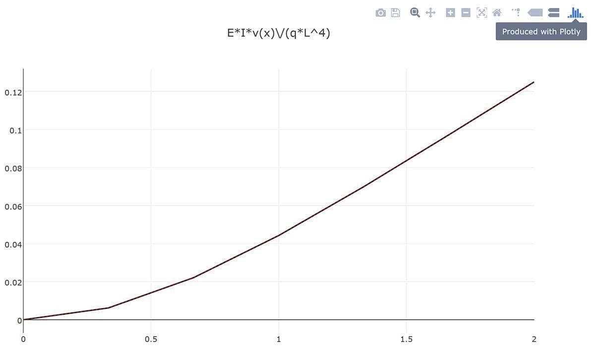
postplot( fea, 'surfexpr', 'E*I*v/(q*L^4)', 'linewidth', 2 ), hold on
postplot( fea, 'surfexpr', 'x^2*(6*L^2-4*L*x+x^2)/24/L^4', 'color', 'r', 'linestyle', ':' )
title( 'E*I*v(x)/(q*L^4)' )

postplot( fea, 'surfexpr', 'E*I*th/(q*L^3)', 'linewidth', 2 ), hold on
postplot( fea, 'surfexpr', 'x*(3*L^2-3*L*x+x^2)/6/L^3', 'color', 'r', 'linestyle', ':' )
title( 'E*I*theta(x)/(q*L^3)' )

postplot( fea, 'surfexpr', 'M/(q*L^2)', 'linewidth', 2 ), hold on
postplot( fea, 'surfexpr', '1/2*(L-x)^2/L^2', 'color', 'r', 'linestyle', ':' )
title( 'M(x)/(q*L^2)' )
Note that due to Octave bugs the postprocessing commands above crash and segfault on the tested systems, an alternative is to use the integrated Plotly html web visualization and posprocessing functionality.
p1 = postplot( fea, 'surfexpr', 'E*I*v/(q*L^4)', 'linewidth', 2, 'renderer', 'plotly' )
p2 = postplot( fea, 'surfexpr', 'x^2*(6*L^2-4*L*x+x^2)/24/L^4', 'color', 'r', 'linestyle', ':', 'renderer', 'plotly' )
p1.data = [ p1.data p2.data ];
plotly_html_file = plotlyoffline( p1 )
Although very hard to discern from the resulting image, the exact and computed solutions agree and perfectly overlap as would be expected here.

Vibration analysis
To perform an vibrational analysis to calculate eigenmodes and eigenfrequencies we use manual assembly to build the input required for the MATLAB eigs function (calling arpack). Here we want to get the mass and stiffness matrices due to
\[ \rho A(x)\frac{\partial^2 v}{\partial t^2} - \frac{\partial^2 }{\partial x^2}(EI(x)\frac{\partial^2 v}{\partial x^2}) = 0 \]
where $\rho$ is the material density, and A the cross-sectional
area. For the problem setup we proceed as above omitting the help
equation for th. To directly compute the matrices we use the
assembleprob function with
flags f_m, f_a, and f_sparse to compute and return the sparse
mass and stiffness matrices
% Parse and assemble matrices.
fea = parseprob( fea );
[M,A] = assembleprob( fea, 'f_m', 1, 'f_a', 1, 'f_sparse', 1, 'icub', 4 );
As for boundary conditions we must here eliminate rows corresponding to the homogeneous Dirichlet ones as
% Eliminate Dirichlet boundary conditions from matrices.
ix_b = ones(size(M,1),1);
[tmp,ix_b] = bdrsetd( [], ix_b, fea );
ix_rem = find(ix_b==0);
M(:,ix_rem) = [];
M(ix_rem,:) = [];
A(:,ix_rem) = [];
A(ix_rem,:) = [];
The problem can now be solved for the desired number of eigenfrequencies by calling the built-in eigs function
% Solve for eigenvalues and eigenvectors.
n_eigs = 6;
[V,D] = eigs( A, M, n_eigs, 0 );
efq = sqrt(diag(D))/(2*pi);
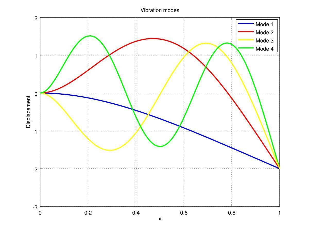
We can also plot and visualize the four first vibration modes as follows
figure, hold on, grid on
cols = {'b' 'r' 'y' 'g' 'c' 'm'};
x = fea.grid.p;
ind_dof_v = find(ix_b(1:length(x)));
for i=1:4
  y = zeros(size(x));
  y(ind_dof_v) = V(1:length(ind_dof_v),n_eigs-i+1);
  plot( x, y, 'color', cols{mod(i-1,6)+1}, 'linewidth', 2 )
end
legend( {'Mode 1' 'Mode 2' 'Mode 3' 'Mode 4'} )
title(  'Vibration modes' )
xlabel( 'x' )
ylabel( 'Displacement' )

The FEATool Multiphysics model m-script files for these two beam simulation examples can be found in the FEATool examples directory as ex_euler_beam1 and ex_euler_beam2.
