When given the task to perform many simulations in a larger simulation study or project, such as in optimization studies or parametric studies over several variables as for example described in a parametric simulation script tutorial, one can speed up the overall process significantly by performing the simulations in parallel. In the following an automated way to accomplish this using the Unix xargs tool with a bash command script is described.
It is both natural and easy to simply run simulations in sequence with for loops, but as modern machines often have multiples of CPU cores available one can significantly reduce the total simulation time running the jobs in parallel. The script described in the following will run on any Linux or Unix machine with bash and xargs installed including Windows systems with the WSL - Ubuntu Bash for Windows Subsystem shell. MATLAB® or GNU Octave is also a requirement for running m-script files.
In the first part of the control script (setup and configuration) the total number of parallel runs and the number of simultaneous number of parallel processes is defined (the latter typically taken as the number or CPU cores or threads available).
#!/bin/bash
n_parruns=16   # Total number of jobs/runs.
n_parproc=3    # Number of simultaneous parallel processes.
Also the path to the Octave or MATLAB binary executable file has to be specified, as well as a MATLAB m-script file to run, in this case simply called mscript.m.
export runcmd='/mnt/c/Octave/Octave-4.2.1/bin/octave-cli.exe'
export mscript=mscript.m
Next a global function is defined which will be called for each parallel run and start its own MATLAB/Octave instance to run a simulation.
function parfun
{
    echo parproc$1-$$: start   # Terminal output.

    # Write parproc file to temporary (current) directory.
    tempdir=$(pwd)
    echo > "$tempdir/parproc$1-$$"

    # Octave/MATLAB command string.
    cmdstr="i_parrun = $1;
            $(sed -n '/exit/!p;//q' $mscript)
            delete([pwd,filesep,'parproc$1-$$']);"

    echo "$cmdstr" > mscript_$1.m
    eval $runcmd" mscript_$1.m"

    # Sleep while parproc file exists.
    while [ -f "$tempdir/parproc$1-$$" ]
    do
        sleep 1
    done

    # Cleanup.
    rm -f mscript_$1.m
    rm -f parproc$1-$$

    echo parproc$1-$$: end   # Terminal output.
}
export -f parfun
Lastly, xargs is called which automatically handles the batch processing, that is to run n_parproc m-scripts in parallel and starting new jobs as running ones have finished.
eval "printf \"%i\n\" {1..$n_parruns}" | xargs -n 1 -P $n_parproc -I {} bash -c 'parfun "$@"' _ {}
The whole script supporting both MATLAB and Octave calls can be downloaded from the following link
As for the m-script file to run, it can contain any valid MATLAB code including FEATool FEM functions (just make sure MATLAB/Octave can find FEATool in the defined paths). The important thing to note is that each instance has access to a variable i_parrun containing the parallel job number (1-n_parruns). This variable can in turn be used to select and set simulation and processing parameters.
For example, the following m-script can be used to run a parametric study of the hole in plate plane-stress model, varying both the hole diameter and plate thickness
disp(['parallel simulation run ',num2str(i_parrun)])

i_cnt = 0;
for diam = [0.01 0.02 0.03 0.05]
  for thick = [0.001 0.0015 0.002 0.004]

    i_cnt = i_cnt + 1;
    if( i_parrun==i_cnt )   % Only run the simulation for i_parrun
      [fea,out] = ex_planestress1( 'diam', diam, 'thick', thick, 'iplot', 0 );
      eval( ['fea',num2str(i_parrun),' = fea;'] )
      save( ['fea',num2str(i_parrun)], ['fea',num2str(i_parrun)] )
    end

  end
end
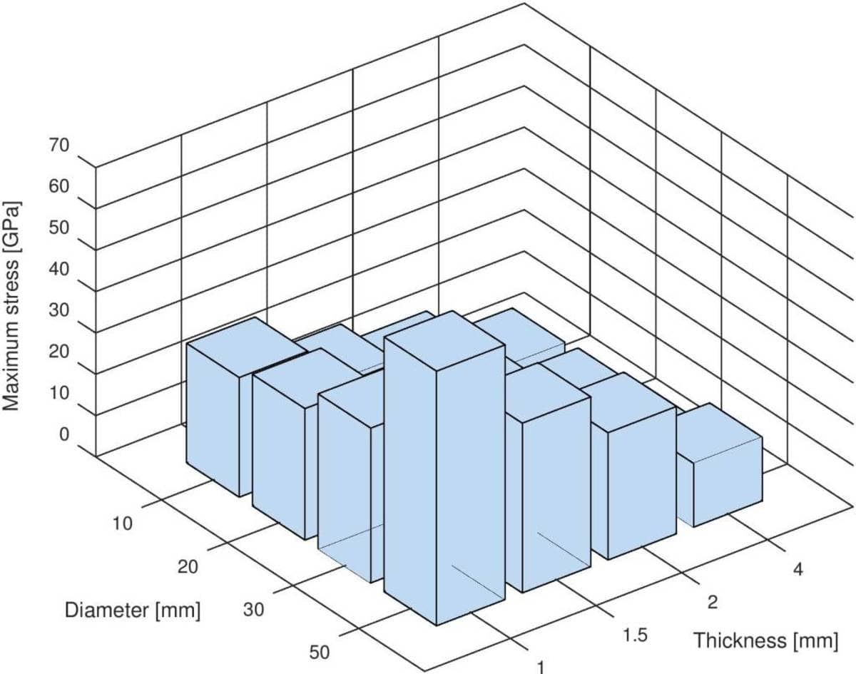
Once all the simulation runs have finished one can collect, postprocess and visualize the results, for example
diam  = [0.01 0.02 0.03 0.05];
thick = [0.001 0.0015 0.002 0.004];
s_sx  = '200e9/(1-0.3^2)*ux + 0.3*200e9*vy';
for i=1:length(diam)
  for j=1:length(thick)
    i_cnt = 4*(i-1) + j;

    load( ['fea',num2str(i_cnt)] )
    eval( ['fea = fea',num2str(i_cnt),';'] )

    [~,sx_max(i,j)] = minmaxsubd( s_sx, fea );
  end
end

bar3(sx_max*1e-6)
xlabel( 'Thickness [mm]' )
set( gca, 'xticklabel', regexp(num2str(thick*1e3),'\s+','split') )
ylabel( 'Diameter [mm]' )
set( gca, 'yticklabel', regexp(num2str(diam*1e3),'\s+','split') )
zlabel( 'Maximum stress [GPa]' )

In this particular case we can see that the maximum stress is found with the largest diameter hole and thinnest plate as expected due to the least amount of material left.