This tutorial builds on and continues the previous CAD and Gmsh file import and mesh generation tutorial. A parametric deformation and stress analysis of the imported fixed wrench and spanner CAD model will be performed with a number of different load configuration cases. The following five steps are all that is required to set up and solve this structural mechanics deformation example in FEATool using both the MATLAB GUI as well as the command line interface (CLI).
1. New Model and Grid Import from External File
Having the previously generated Gmsh grid, the first step is to start a new 3D model with the Linear Elasticity physics mode selected. As an external grid will be imported it is not necessary to create a geometry (FEATool geometries are only used by the built-in gridgen function for meshing and grid generation).
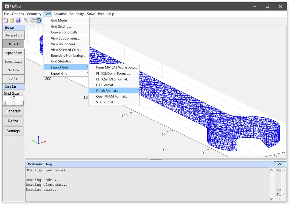
Switch to Grid mode and import the spanner.msh Gmsh grid file (click on the link to
download) into the FEATool GUI by selecting the Import Grid >
Gmsh Format option found in the Grid menu.
2. Equation Settings
Switching to Equation mode automatically opens the Equation
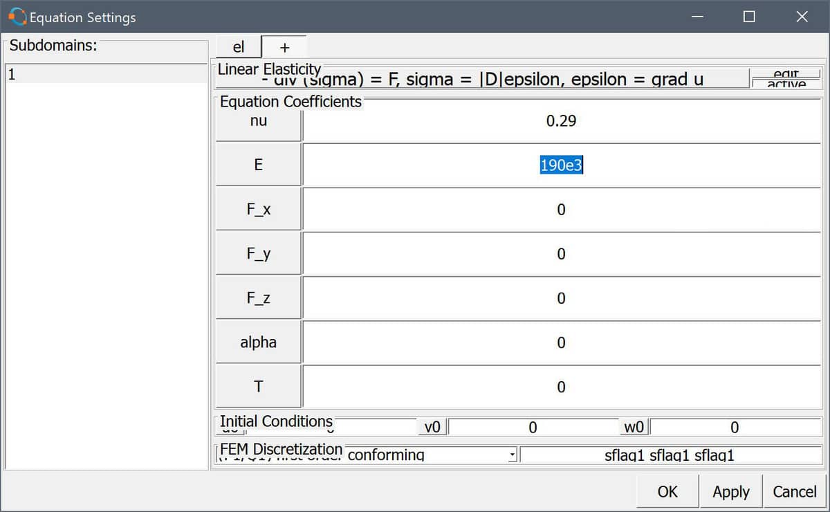
Settings dialog box. There the material parameters can be
prescribed, in this case a Poisson ratio of 0.29, and modulus of
elasticity of 190e3 N/mm is used, which corresponds to tool
chromium-vanadium grade steel alloy (scaled to mm units since the
geometry is given in millimeters, to convert to meter units one can
scale the grid vertex coordinates as fea.grid.p =
fea.grid.p*1e-3; ).
3. Boundary Conditions
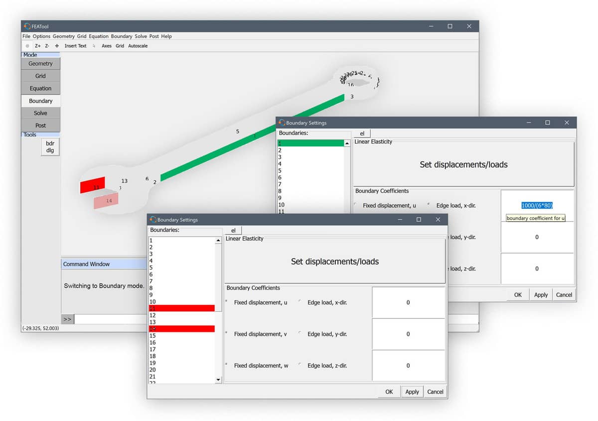
Switch to Boundary mode to prescribe loads and displacements. First, select all boundaries in the Boundary Settings dialog box, prescribe zero Edge loads in all directions, and press Apply. This will set all boundaries free by default (the Ctrl+a key combination can be used to select all items in list selection boxes such as for geometry objects, boundaries, and subdomains).
For this model the flat surfaces at the front fork are assumed to be fixed (by wrapping around an fixed and immobile bolt). To do this select boundaries 13 and 14, and choose fixed displacement conditions in all directions.
Lastly, select one of the side boundaries (here number 4) and enter the force expression -1000/(6*80)*(y>140) for the Edge load, x-dir. to apply a pulling force of 1000 N over an area of 6*80 mm at the top half of the handle (y > 140 mm). Here the switch expression y>140 will evaluate to 1 if true and 0 if false, and in this way it is possible to localize and activate equation and boundary coefficients without having separate discrete boundaries or subdomains.
4. Solution and Postprocessing
To solve the model change to Solve mode and press the
= button. After the solution has been computed FEATool
switches to Postprocessing mode and displays the default solution
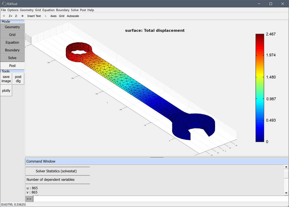
plot. Open the Postprocessing Settings dialog box and choose
Surface Plot with the Total Displacement as surface
expression. As can be seen below the maximum displacement in this case
is about 2.5 mm towards the ring end of the wrench.
5. Parametric Study
In order to perform a parametric study, the model can be saved as a
MATLAB m-file script using the Save As M-Script Model…
option found in the File menu. The script can be opened
and edited in a text editor.
In the following the model has been set up and changed to shift the load from the strong in-plane x-direction to the weaker lateral z-direction by introducing the parameter frac. For postprocessing a deformed grid will be computed and displayed.
% Fraction of lateral to inline force distribution 0..1
frac = linspace(0,1,200);

% Import Gmsh CAD grid.
fea.sdim = {'x','y','z'};
fea.grid = impexp_gmsh( 'spanner.msh', 'import' );

% Add 3D solid linear elasticity physics mode
% and define material parameters.
fea = addphys( fea, @linearelasticity );
fea.phys.el.eqn.coef{1,end} = { 0.29  };
fea.phys.el.eqn.coef{2,end} = { 190e3 };

% Set all boundaries to no load per default.
n_bdr  = max(fea.grid.b(3,:));
bc_sel = cell(3,n_bdr);
[bc_sel{:}] = deal(0);

% Fix all displacements on boundaries 11 and 14.
[bc_sel{:,[11 14]}] = deal(1);
fea.phys.el.bdr.coef{5} = bc_sel;


% Main loop.
fea = parsephys(fea);
fea = parseprob(fea);
for i=1:length(frac)

  % Split forces in x/z-directions according to frac.
  fea.bdr.n{1}{1} = ['-',num2str((1-frac(i))*1000/(6*80)),'*(y>140)'];
  fea.bdr.n{3}{4} = [    num2str(   frac(i) *1000/(6*80)),'*(y>140)'];

  % Solve problem.
  fea.sol.u = solvestat( fea );

  % Create fea struct with displaced grid.
  dp = zeros(size(fea.grid.p));
  for j=1:3
    dp(j,:) = 2*evalexpr( fea.dvar{j}, fea.grid.p, fea );
  end
  fea_disp = fea;
  fea_disp.grid.p = fea_disp.grid.p + dp;

  % Plot deformed object colored by the total displacement.
  clf
  postplot( fea_disp, 'surfexpr', 'sqrt(u^2+v^2+w^2)', ...
            'colorbar', false, 'linewidth', 0.1 )
  view( [-60 20] ), axis off

  pause
end
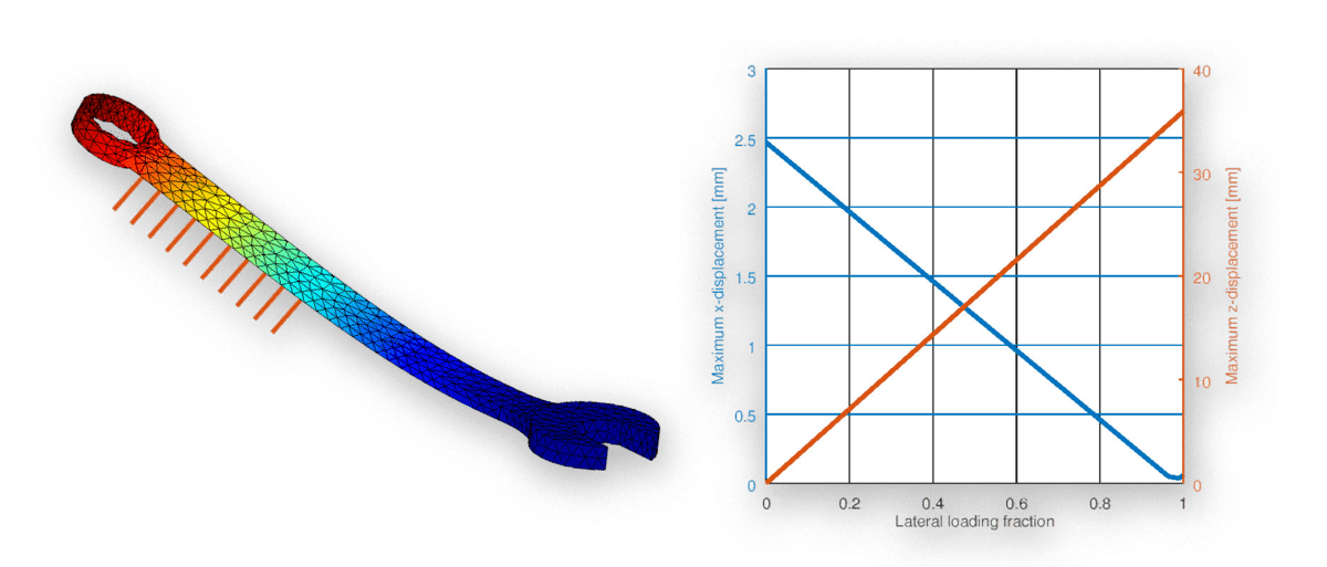
After running the parametric script and looking at the results one can see that the maximum deformation has increased from 2.5 mm with in-plane loading to almost 4 cm with lateral plane loading. Although, this large deformation most certainly violates the linear elastic deformation assumption, it is still a useful example showing how easy and fast it is to define and set up automated parametric studies with FEATool and MATLAB m-file scripts.
The complete parametric structural mechanics study of a fixed spanner, including advanced postprocessing, can be downloaded from the following link (while the actual wrench Gmsh grid file can be downloaded from the link above).