Using Mixed Robin Boundary Conditions in FEATool

Robin boundary conditions or mixed Dirichlet (prescribed value) and Neumann (flux) conditions are a third type of boundary condition that for example can be used to implement convective heat transfer and electromagnetic impedance boundary conditions. In the following it will be discussed how mixed Robin conditions are implemented and treated in FEATool with an illustrative example (in short Robin conditions can be entered in FEATool as the usual Neumann flux coefficients).

Consider the following one-dimensional convection, diffusion, and reaction model example

\[ \frac{\partial^2 u}{\partial x^2} + u\frac{\partial u}{\partial x} - u = e^{2x} \]

with the two boundary conditions

\[ \left\{\begin{aligned} u+\frac{\partial u}{\partial x} = 2 &, \qquad x = 0\\\
u = e &, \qquad x = 1 \end{aligned}\right. \]

and the exact solution $u(x) = e^x$.

The first boundary condition $u+\frac{\partial u}{\partial x} = 2$ at $x=0$ is of the mixed Robin type, prescribing a combination of both the solution value (Dirichlet) and gradient or flux (Neumann). Rewriting it as $\frac{\partial u}{\partial x} = 2-u$ one can see that it can be formulated as a Neumann boundary coefficient ($\frac{\partial u}{\partial x} = g$). The second boundary condition at $x=1$ is of the usual Dirichlet prescribed value type.

This example problem can be set up and implemented in the FEATool MATLAB m-script language as follows. First, a 1D domain is defined with x as the space coordinate name. The dependent variable is named u and assigned first order linear FEM shape functions sflag1. Furthermore, a one dimensional mesh with 10 grid cells spanning $x=0$ to $x=1$ is created with the linegrid command.

fea.sdim  = {'x'};
fea.dvar  = {'u'};
fea.sfun  = {'sflag1'};
fea.grid  = linegrid(10,0,1);

Although one could use the pre-defined convection and diffusion, Poisson, or custom equation modes to define the governing PDE equation, here it is manually and explicitly defined as ux_x + uux_t - u_t = exp(2x). The parseeqn function checks and parses the equation to the weak finite element syntax stored in the fea.eqn field. For convenience a coefficient expression is also defined for the analytic reference solution.

fea.eqn   = parseeqn( 'ux_x + u*ux_t - u_t = exp(2*x)', ...
                      fea.dvar, fea.sdim );
fea.coef  = {'u_ref', 'exp(x)'};

The _x and _t underscore syntax means that the terms will be evaluated and assembled implicitly as bilinear forms. If the underscores (and _t test functions) are omitted the terms will be evaluated explicitly and the problem will become more non-linear.

The Dirichlet boundary condition should be defined for $x=1$, the second and last boundary point, where the exact solution is prescribed (in the fea.bdr.d boundary coefficient field, the first entry is left empty as no Dirichlet conditions is to be applied there).

fea.bdr.d = {[],'u_ref'};

As the fist point at $x=0$ the Robin boundary 2-u condition is defined as a Neumann condition (in the fea.bdr.n boundary coefficient field).

fea.bdr.n = {'2-u',[]};

Lastly, parsing, solving and postprocessing can be done with the commands

fea = parseprob(fea);
fea.sol.u = solvestat(fea);

h1 = postplot( fea, 'surfexpr', 'u', 'color', 'b' );
h2 = postplot( fea, 'surfexpr', 'u_ref', ...
                    'linestyle', '--', 'color', 'r' );

legend( [h1(1),h2(1)], 'computed solution', ...
                       'analytic solution' )
xlabel('x')
ylabel('u')
grid on

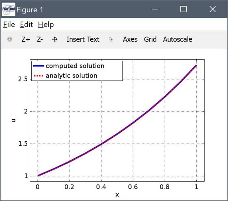
The plot and image below clearly shows how the computed solution aligns with the analytic reference solution.

Note that the solver will call the bdrneu FEATool function during the solution process to analyze the fea.bdr.n field, and try to automatically split Robin conditions into Neumann and Dirichlet parts for separate treatment. In this example the Neumann contribution 2 will be assembled and added explicitly to the right hand side, while the Dirichlet part -u will added implicitly to the corresponding boundary nodes of the stiffness matrix.

The limitation for FEATool to be able to parse Robin conditions is that the linear Dirichlet part must be easily identifiable. If for example the Robin expression is implemented as a coefficient expression, then a Robin dependent variable cannot be identified and the whole expression will be evaluated explicitly. This can be seen by making the following changes to the model problem, where although an identical solution is achieved, the solver takes more iterations to converge as the problem is more nonlinear with the explicit evaluation of the Robin boundary condition.

fea.bdr.n = {'robin_bc',[]};
fea.coef  = {'u_ref', 'exp(x)';
             'robin_bc', '2-u'};
fea.sol.u = solvestat( fea, 'maxnit', 50 );
postplot( fea, 'surfexpr', 'u', 'color', 'g', 'linestyle', '-.' );

This model example is available as ex_robinbc1.m in the FEATool examples directory

Although the model example here has been implemented using the FEATool functions and MATLAB m-script language on the command line, Robin boundary can similarly be used in the FEATool GUI by entering valid Robin expressions in the corresponding Neumann or flux boundary coefficient edit fields.