Featuring an easy to use graphical user interface (GUI), FEATool Multiphysics is also fully compatible with MATLAB functions and its scripting language. As simulation models both can be saved in a binary format and also as m-script language files, FEATool can therefore be used with all built-in MATLAB functionality as well as with Simulink and the Optimization Mathworks toolboxes.
Closely related to the article on parameter search and optimization in FEA physics simulations using the fzero MATLAB function, the following post illustrates how to integrate and use the fminbnd minimization function with a finite element FEA simulation model to conduct a quick and simple parameter search.
The example CFD problem used in the following considers two-dimensional potential flow around a solid object with the stream-function formulation, that is
where the velocities are defined as u = -∂ψ/∂y and v = ∂ψ/∂x. Appropriate boundary conditions include prescribed stream-function or free stream velocity on the external boundary, and a prescribed constant stream-function value on the body. If both the flow field and body shape are symmetric then the value of the stream-function is zero on the body. However, for non-symmetric flows and bodies the stream-function should be non-zero in order to correct for non-physical flow field effects.
The issue is that at the sharp trailing edge of an airfoil or wing profile the velocity should be either zero or continuous in the normal direction of the flow field according to the Kutta condition. This can be achieved by offsetting the stream-function on the boundary of the airfoil. This phenomena is illustrated in the figure below.
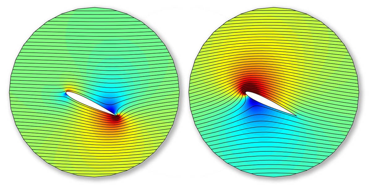
In the left side simulation the flow field curls around the trailing edge and features an unphysical stagnation point on the top of the airfoil. In contrast, the results of the corrected right hand side simulation show a continuous flow field and streamlines from the trailing edge.
Although ineffective, one can use trial and error to find the actual value and corrected value of the stream-function at the boundary of the body. A better approach is to recognize that what we actually are looking for, is to find the stream-function value on the body for which the velocity at the trailing edge is zero or minimized. As the magnitude of the velocity U = √(u2+v2) will always be positive (and possibly not even numerically zero), the fzero function can not be used. Instead the fminbnd and potentially also fminsearch MATLAB functions are appropriate here, and works in the same way as fzero.
Define a MATLAB function that takes a one parameter argument, in this case the steam-function at the body, and returns the velocity magnitude at the trailing edge. The problem function in this example is defined as an anonymous function, but could just as well be implemented as a regular MATLAB function.
pfun = @(psi_body) velocity_at_trailing_edge(psi_body);
This function which constructs and solves the potential flow problem is then called by fminbnd with lower and upper limits on psi
found_psi_body = fminbnd( pfun, psi_min, psi_max );
Running the script for a NACA 0012 wing profile at a 6 degree angle of attack, we find that fminbnd takes 11 tries in the search and successfully narrows down the stream-function value to -0.178 yielding a minimum velocity magnitude at the trailing edge of 0.78234.
>> ex_potential_flow1

 Func-count     x          f(x)         Procedure
    1       -2.36068       23.541        initial
    2        2.36068      27.3679        golden
    3       -5.27864      54.9821        golden
    4      -0.267231      1.24343        parabolic
    5     -0.0929204      1.20285        parabolic
    6      -0.154739     0.821156        parabolic
    7      -0.178032     0.783252        parabolic
    8      -0.181615      0.78442        parabolic
    9      -0.177581      0.78324        parabolic
   10      -0.177624      0.78324        parabolic
   11      -0.177658      0.78324        parabolic

Optimization terminated:
the current x satisfies the termination criteria using OPTIONS.TolX of 1.000000e-04
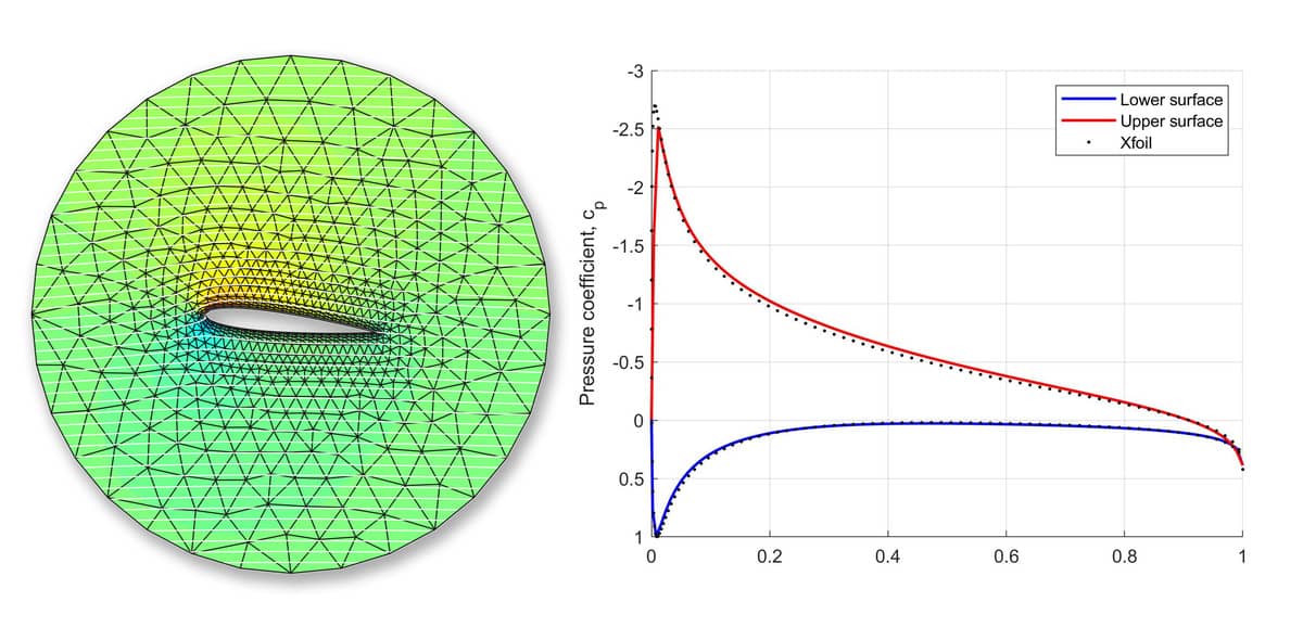
As shown in the figure below, the solution and resulting pressure coefficient cp is in well agreement with computations using XFoil and panel methods. (In order to increase the accuracy in the boundary region the computational grid also uses the boundary layer available with the gridgen mesh generator).
The entire MATLAB m-script model file can be downloaded from the link below
Note that fminbnd will call both the FEA definition function and solver in each minimization step which can become computationally expensive for larger simulations. As done in the example it is advisable to save and reuse as much data as possible, with the persistent MATLAB argument, using old solutions as initial guesses, or pre-computing and caching as much as possible.
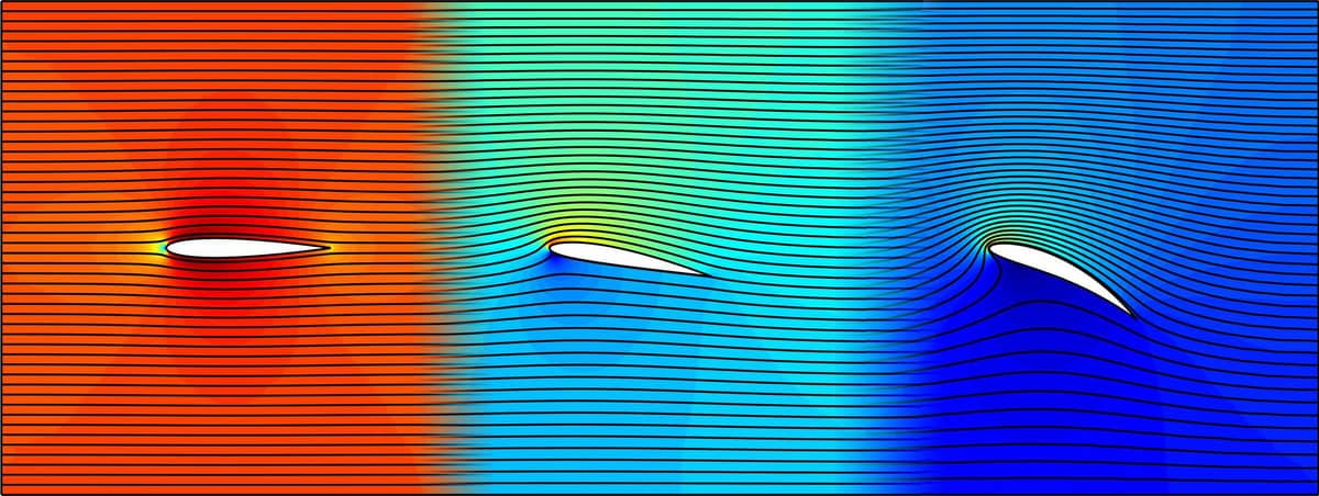
A parametric study showing how the correction for the Kutta condition
effects the flow field for a NACA 4415 wing profile at 0 to 30 degrees
of angle of attack, can be seen in the video below.
Additional examples featuring optimization and parameter search can be found in the topology optimization example, and more on m-file script models can also be seen in the parametric study of the deflection of a bracket and bending of a wrench models and tutorials.