Conducting Sphere

This verification example considers a perfectly conducting sphere placed between two charged capacitor plates. An axisymmetric solution for the electrostatic potential is compared with a full 3D one, and verified against the analytical solution U(x_i) = E₀*(r³/x_i² - x_i), where the electrical field is the potential difference divided by the distance between the plates E_i = dV/d_i.

In this example the conductive sphere is given a radius of 1 mm while the distance between the places is 1 cm. The area of the places is taken as 0.1 x 0.1 m and in axisymmetric coordinates a circle with equivalent area. The applied voltage is 20 V and dielectric permittivity of the medium ε = 5.

This model is available as an automated tutorial by selecting Model Examples and Tutorials... > Electromagnetics > Conducting Sphere from the File menu. Or alternatively, follow the step-by-step instructions below.

Tutorial

This model is available as an automated tutorial by selecting Model Examples and Tutorials... > Electromagnetics > Conducting Sphere from the File menu. Or alternatively, follow the step-by-step instructions below.

The axisymmetric case is considered first.

1. To start a new model click the New Model toolbar button, or select New Model... from the File menu.
2. Select the Axisymmetry radio button.

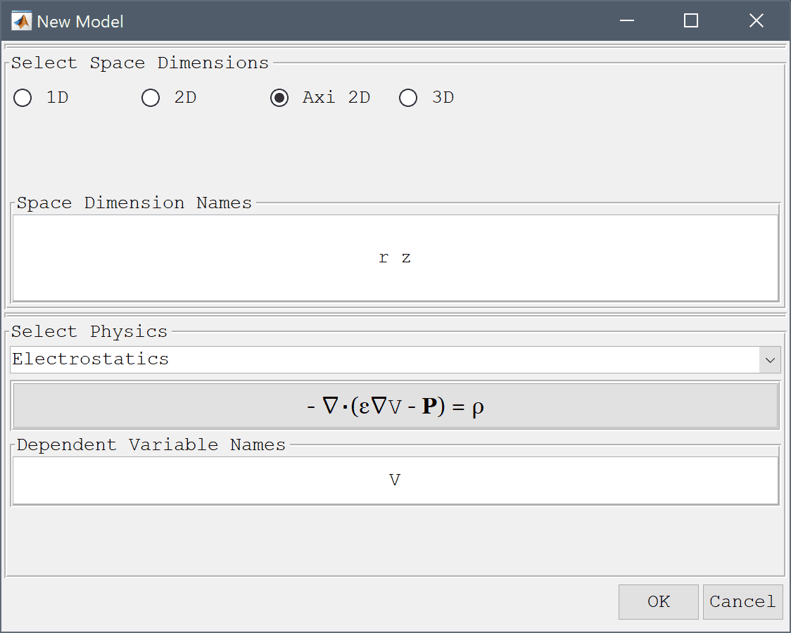
3. Select the Electrostatics physics mode from the Select Physics drop-down menu.

   
4. Press OK to finish the physics mode selection.
5. Select Circle from the Geometry menu.
6. Enter 1e-3 into the radius edit field.
7. Press OK to finish and close the dialog box.
8. Select Rectangle from the Geometry menu.
9. Enter -1e-3 into the x_min edit field.
10. Enter 0 into the x_max edit field.
11. Enter -1e-3 into the y_min edit field.

12. Enter 1e-3 into the y_max edit field.

    
13. Press OK to finish and close the dialog box.
14. Select C1 and R1 in the geometry object Selection list box.
15. Press the - / Subtract geometry objects Toolbar button.
16. Select Rectangle from the Geometry menu.

The max domain radius can be calculated to be 0.0056419 m to have an equivalent area of 1 cm squared.

1. Enter 0 into the x_min edit field.
2. Enter 0.0056419 into the x_max edit field.
3. Enter -0.005 into the y_min edit field.

4. Enter 0.005 into the y_max edit field.

   

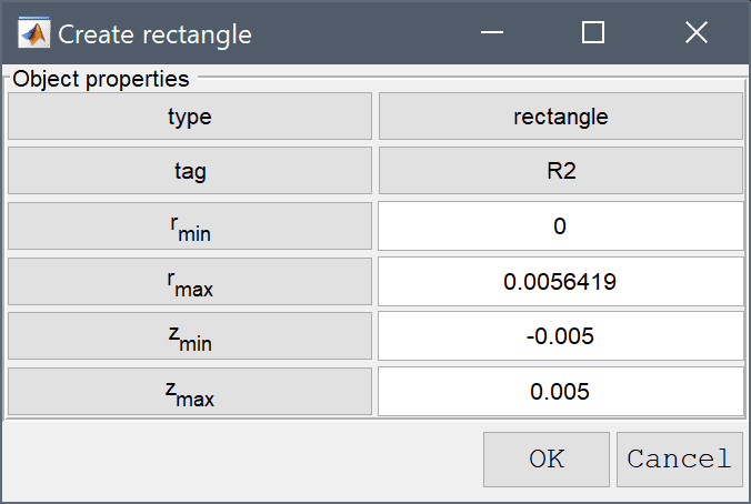
5. Press OK to finish and close the dialog box.

   
6. Switch to Grid mode by clicking on the corresponding Mode Toolbar button.

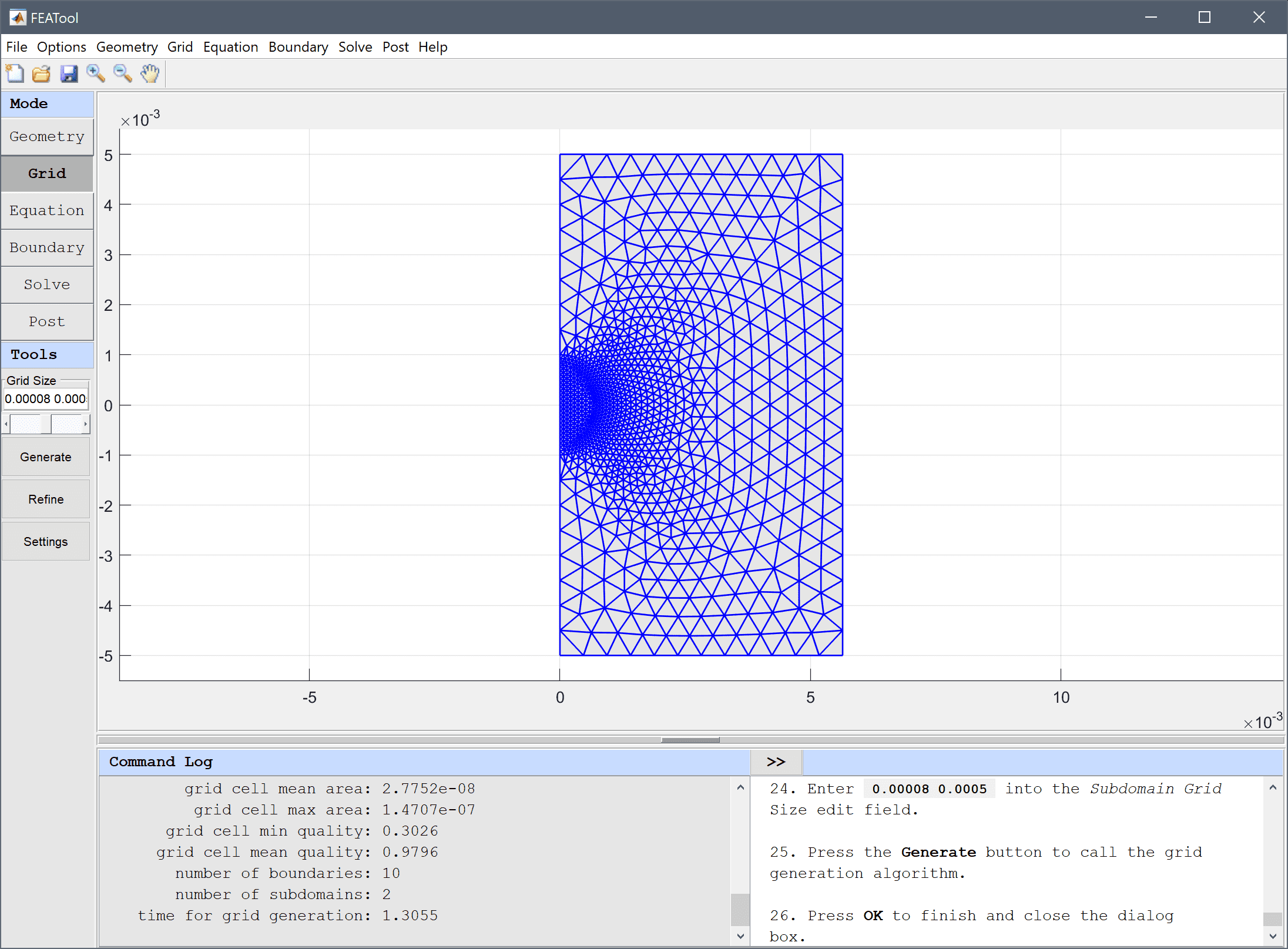
We can prescribe different grid sizes for different subdomains and boundaries. Here a smaller size is used for the sphere domain to locally increase the resolution and accuracy of the simulation.

1. Press the Settings Toolbar button.
2. Enter 0.00008 0.0005 into the Subdomain Grid Size edit field.

3. Press the Generate button to call the grid generation algorithm.

   

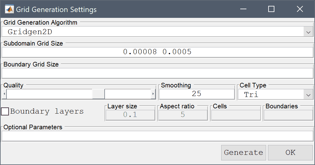
4. Press OK to finish and close the dialog box.

   
5. Switch to Equation mode by clicking on the corresponding Mode Toolbar button.
6. Select 1 in the Subdomains list box.

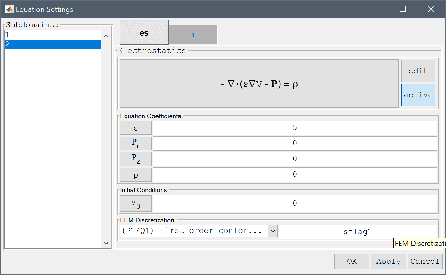
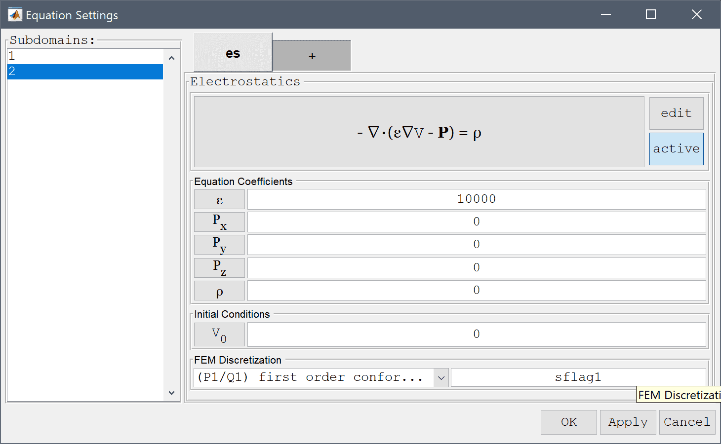
A domain with a very high permittivity can be used to represent a perfectly conducting region.

1. Enter 10000 into the Permittivity edit field.
2. Select 2 in the Subdomains list box.

3. Enter 5 into the Permittivity edit field.

   
4. Press OK to finish the equation and subdomain settings specification.
5. Switch to Boundary mode by clicking on the corresponding Mode Toolbar button.
6. Select 1, 3, 5, and 6 in the Boundaries list box.
7. Select Insulation/symmetry from the Electrostatics drop-down menu.
8. Select 4 in the Boundaries list box.
9. Select Electric potential from the Electrostatics drop-down menu.

10. Enter 12 into the Electric potential edit field.

    
11. Select 2 in the Boundaries list box.
12. Select Electric potential from the Electrostatics drop-down menu.
13. Enter -12 into the Electric potential edit field.
14. Press OK to finish the boundary condition specification.
15. Switch to Solve mode by clicking on the corresponding Mode Toolbar button.
16. Press the = Toolbar button to call the solver. After the problem has been solved FEATool will automatically switch to postprocessing mode and plot the computed solution.

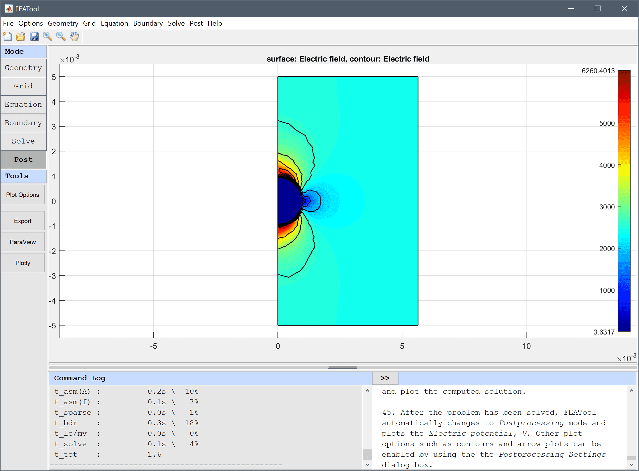
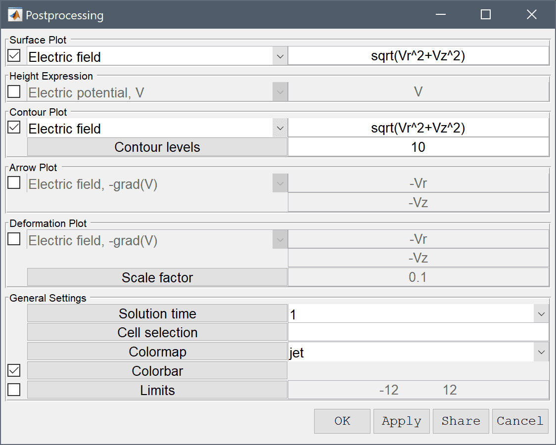
17. After the problem has been solved, FEATool automatically changes to Postprocessing mode and plot the Electric potential, V. Other plot options such as contour and arrow plots can be enabled by using the Postprocessing Settings dialog box.

    
    

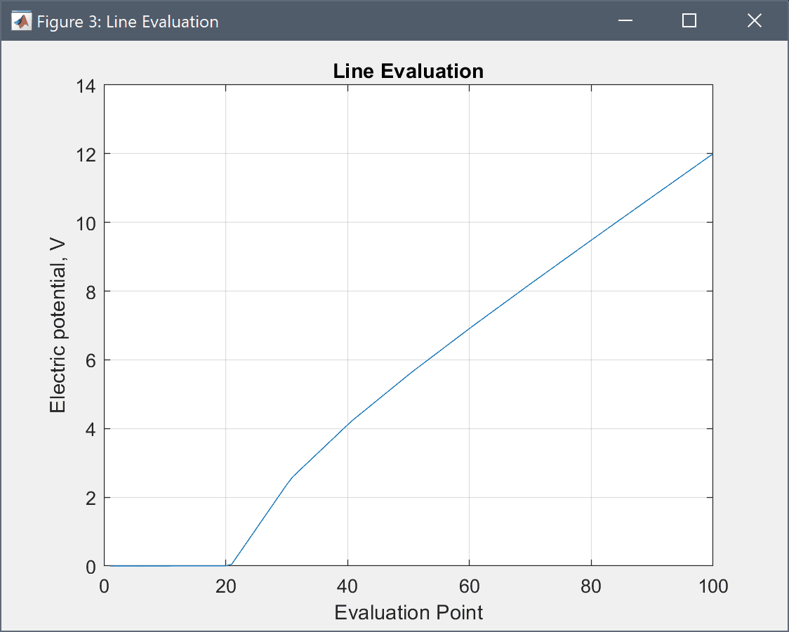
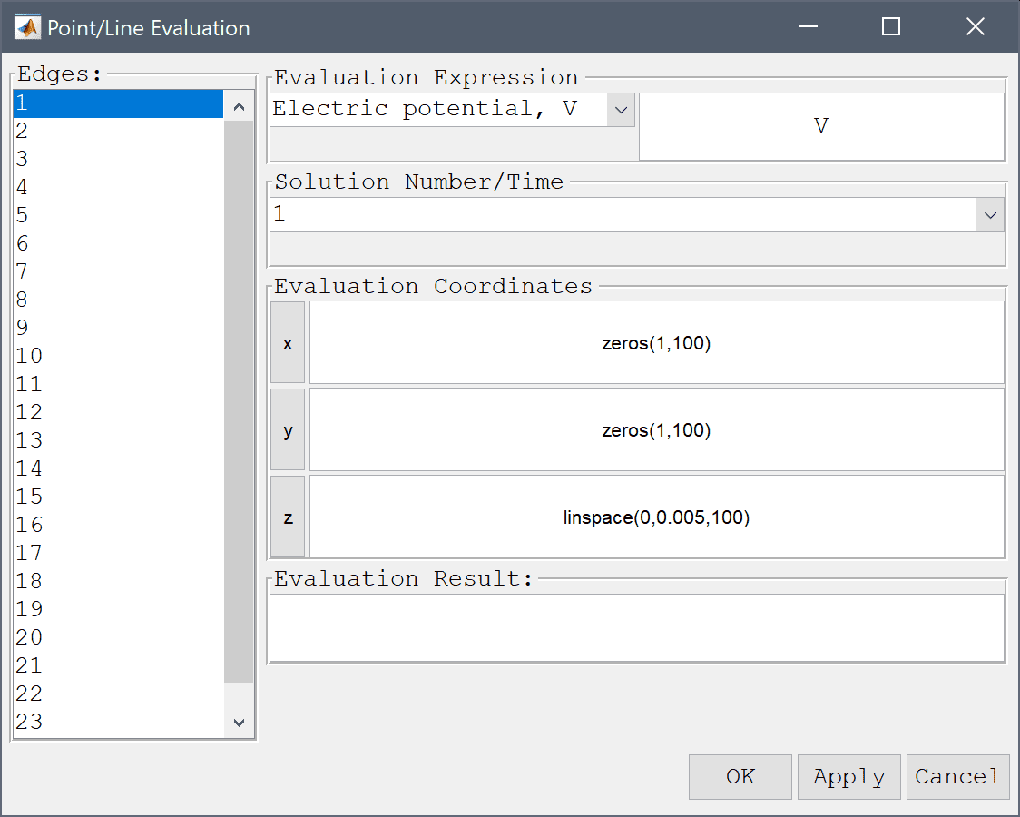
Use the Line Evaluation postprocessing tool to plot the potential as a function of the radius.

1. Select Point/Line Evaluation... from the Post menu.
2. Select Electric potential, V from the Evaluation Expression drop-down menu.

The coordinates can be prescribed as a space or comma separated list of points, or a valid MATLAB expression resulting in a numeric scalar or vector.

1. Enter zeros(1,100) into the Evaluation coordinates in r-direction edit field.

2. Enter linspace(0,0.005,100) into the Evaluation coordinates in z-direction edit field.

   

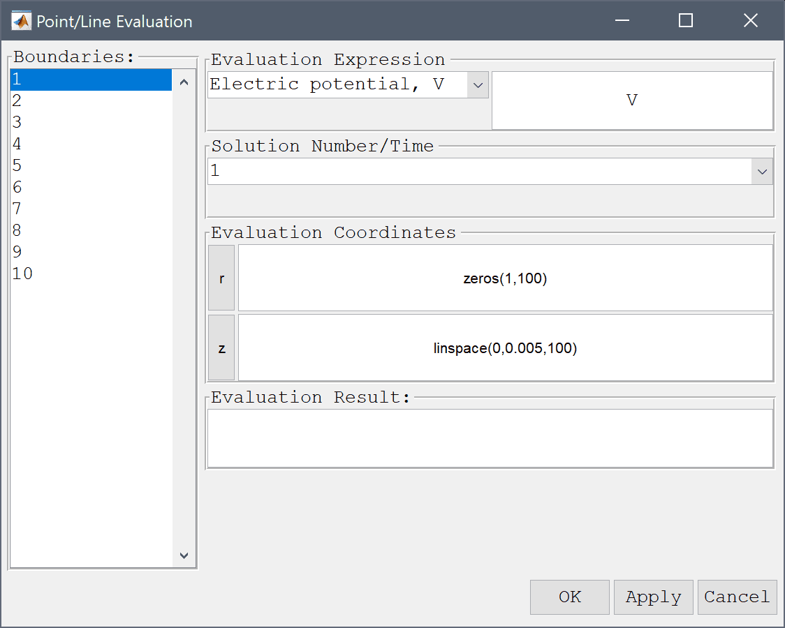
3. Press the Apply button.

   

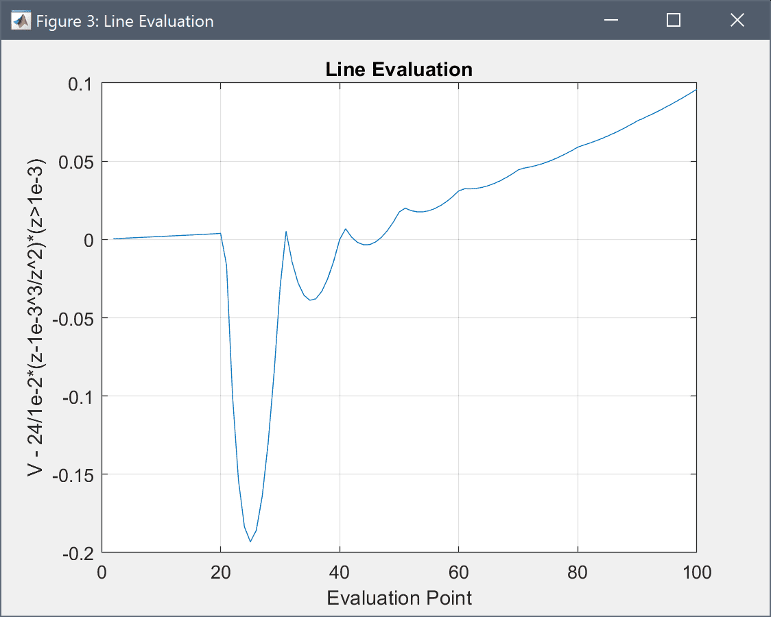
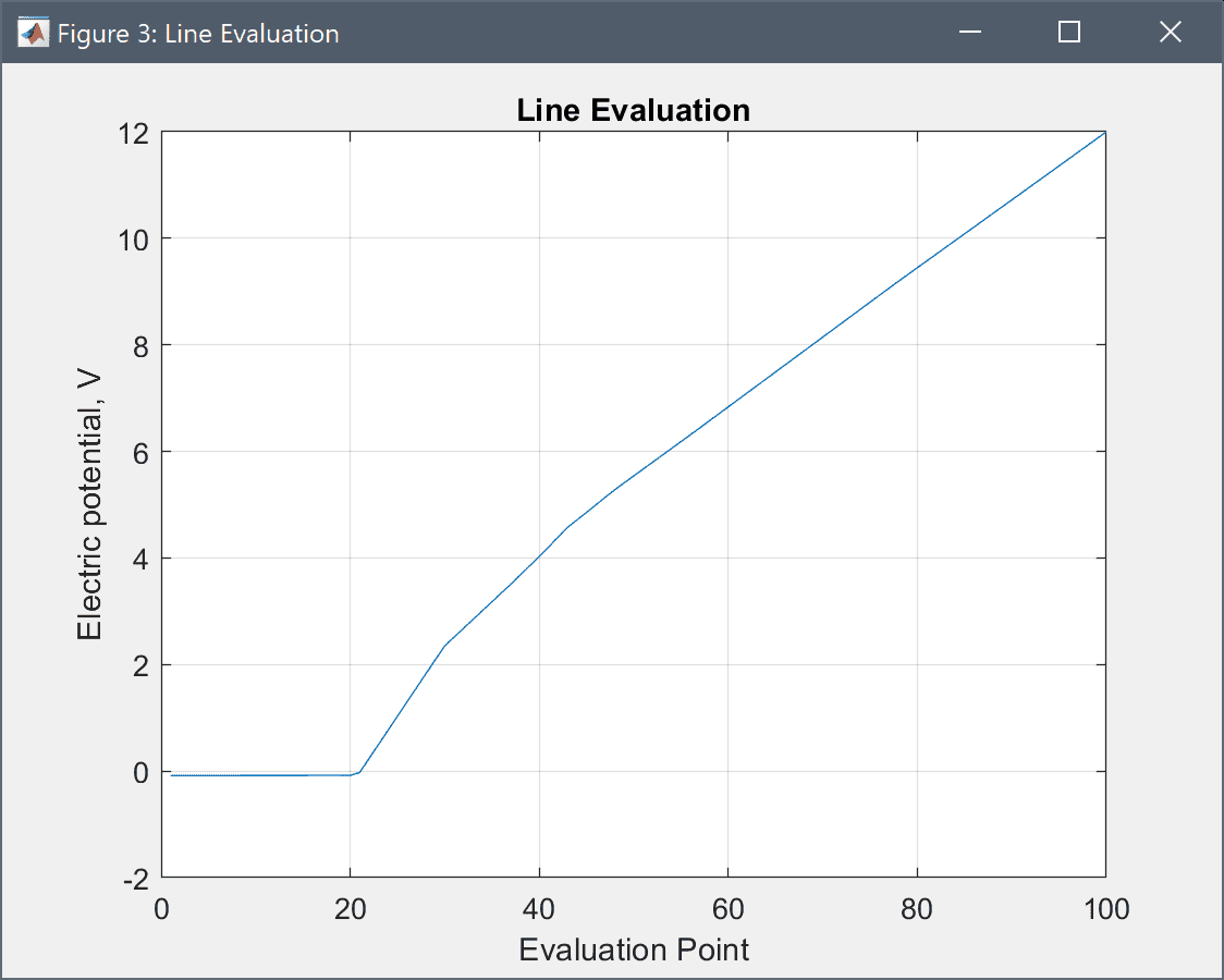
By plotting the difference between the computed potential and the analytical solution we can see how accurate the simulation is. Here we get a maximum error of about 0.1-0.2 V.

1. Enter V - 24/1e-2*(z-1e-3^3/z^2)*(z>1e-3) into the edit field.

2. Press the Apply button.

   
3. Press the Cancel button to close the dialog box.

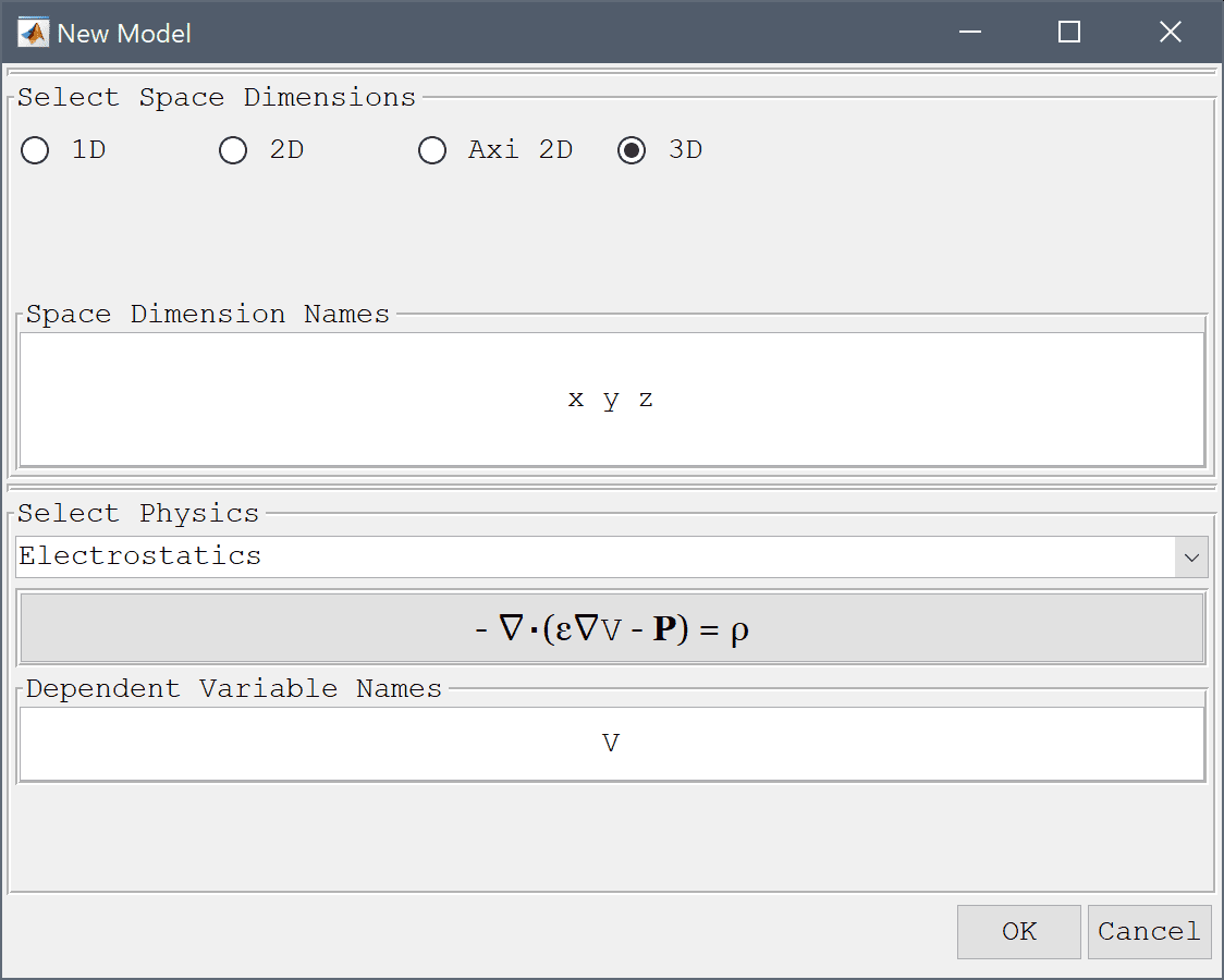
Next we switch to the equivalent model in full 3D with a block domain. The rest of the model setup is analogous to the axisymmetric case.

1. To start a new model click the New Model toolbar button, or select New Model... from the File menu.
2. Select the 3D radio button.

3. Select the Electrostatics physics mode from the Select Physics drop-down menu.

   
4. Press OK to finish the physics mode selection.
5. Press the Create cube/block Toolbar button.
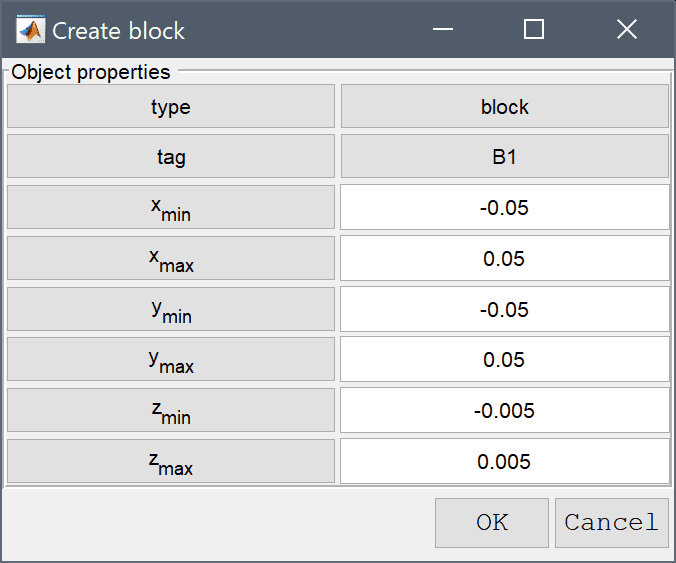
6. Enter -0.05 into the x_min edit field.
7. Enter 0.05 into the x_max edit field.
8. Enter -0.05 into the y_min edit field.
9. Enter 0.05 into the y_max edit field.
10. Enter -0.005 into the z_min edit field.

11. Enter 0.005 into the z_max edit field.

    
12. Press OK to finish and close the dialog box.
13. Select Sphere from the Geometry menu.

14. Enter 1e-3 into the radius edit field.

    

15. Press OK to finish and close the dialog box.

    
16. Switch to Grid mode by clicking on the corresponding Mode Toolbar button.
17. Press the Settings Toolbar button.
18. Enter 0.0002 0.0025 into the Subdomain Grid Size edit field.

19. Press the Generate button to call the grid generation algorithm.

    
20. Switch to Equation mode by clicking on the corresponding Mode Toolbar button.
21. Select 1 in the Subdomains list box.
22. Enter 5 into the Permittivity edit field.
23. Select 2 in the Subdomains list box.

24. Enter 10000 into the Permittivity edit field.

    
25. Press OK to finish the equation and subdomain settings specification.
26. Switch to Boundary mode by clicking on the corresponding Mode Toolbar button.
27. Select 2, 3, 4, and 5 in the Boundaries list box.
28. Select Insulation/symmetry from the Electrostatics drop-down menu.
29. Select 6 in the Boundaries list box.
30. Select Electric potential from the Electrostatics drop-down menu.

31. Enter 12 into the Electric potential edit field.

    
32. Select 1 in the Boundaries list box.
33. Select Electric potential from the Electrostatics drop-down menu.
34. Enter -12 into the Electric potential edit field.
35. Press OK to finish the boundary condition specification.
36. Switch to Solve mode by clicking on the corresponding Mode Toolbar button.
37. Press the = Toolbar button to call the solver. After the problem has been solved FEATool will automatically switch to postprocessing mode and plot the computed solution.
38. Press the Plot Options Toolbar button.
39. Clear the Surface Plot check box.
40. Select the Slice Plot check box.
41. Press OK to plot and visualize the selected postprocessing options.
42. Select Point/Line Evaluation... from the Post menu.
43. Select Electric potential, V from the Evaluation Expression drop-down menu.
44. Enter zeros(1,100) into the Evaluation coordinates in x-direction edit field.
45. Enter zeros(1,100) into the Evaluation coordinates in y-direction edit field.

46. Enter linspace(0,0.005,100) into the Evaluation coordinates in z-direction edit field.

    
47. . Press the Apply button.

The computed 3D potential is very similar to both the axisymmetric and analytic cases as expected.

1. . Enter V - 24/1e-2*(z-1e-3^3/z^2)*(z>1e-3) into the edit field.
2. . Press the Apply button.

The computed errors also show good agreement but could be improved with a finer grid and a higher order approximation.

1. . Press the Cancel button to close the dialog box.

The conducting sphere electromagnetics model has now been completed and can be saved as a binary (.fea) model file, or exported as a programmable MATLAB m-script text file, or GUI script (.fes) file.

CLI Postprocessing

To visualize the full 3D solution from the axisymmetic model, the data can be exported and processed on the MATLAB command line interface (CLI) console with the Export Model Data Struct to MATLAB option from the File menu. The postrevolve and postplot functions can then be applied to revolve and visualize the data, for example

fea_revolved = postrevolve( fea, 24, 0.6 );

% Note that the r-coordinate is replaced by
% "x" in the revolved 3D fea data struct
postplot( fea_revolved, 'surfexpr', 'sqrt(Vx^2+Vz^2)', ...
          'parent', figure, 'axis', 'off', 'colorbar', 'off' )
view(0, 25)