Supersonic Flow Over an Obstacle

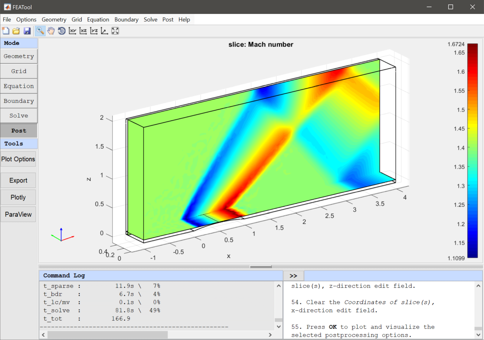
In this example, we simulate three-dimensional supersonic flow through a straight channel with a small obstacle on one wall. The obstacle could represent anything from a protrusion on an aircraft wing to a structural feature in a pipe, like for example in scenarios involving high-speed aircraft or rocket exhausts.

When the high speed flow (Ma = 1.4) impacts the obstacle shock waves are generated and diffracted from both the obstacle and channel walls (that is abrupt and sharp changes in pressure, temperature, and density). This simulation is based on a two-dimensional reference case using the inviscid compressible Euler equations, which has been extensively studied for compressible flow in previous research [1].

Tutorial

This model is available as an automated tutorial by selecting Model Examples and Tutorials... > Fluid Dynamics > Supersonic Flow over an Obstacle from the File menu. Or alternatively, follow the step-by-step instructions below.

Note that the CFDTool interface differ slightly from the FEATool Multiphysics instructions described in the following.

1. To start a new model click the New Model toolbar button, or select New Model... from the File menu.
2. Select the 3D radio button.
3. Select the Euler Equations physics mode from the Select Physics drop-down menu. (Note that for CFDTool the physics selection is done in the Equation settings dialog box.)
4. Press OK to finish the physics mode selection.
5. Press the Create cube/block Toolbar button.
6. Enter -1 into the x_min edit field.
7. Enter 4 into the x_max edit field.
8. Enter 0.5 into the y_max edit field.
9. Enter 2 into the z_max edit field.
10. Press OK to finish and close the dialog box.
11. To create a cylinder, first click on the Create cylinder/cone Toolbar button.
12. Enter 0.5 0 0.042-(0.5^2/0.042+0.042)/2 into the center edit field.
13. Enter (0.5^2/0.042+0.042)/2 into the radius₁ and radius₂ edit fields.
14. Enter 0.5 into the length edit field.
15. Enter 0 1 0 into the axis edit field.
16. Press OK to finish and close the dialog box.
17. Select Combine Objects... from the Geometry menu.
18. Enter B1-C1 into the Geometry Formula edit field.
19. Press OK to finish and close the dialog box.
20. Switch to Grid mode by clicking on the corresponding Mode Toolbar button.
21. Enter 0.08 into the Grid Size edit field.
22. Press the Generate button to call the grid generation algorithm.
23. Switch to Equation mode by clicking on the corresponding Mode Toolbar button. (Note that the Equation Settings dialog box may look different for CFDTool.)
24. Enter rho0 into the Initial condition for rho edit field.
25. Enter u0 into the Initial condition for u edit field.
26. Enter v0 into the Initial condition for v edit field.
27. Enter w0 into the Initial condition for w edit field.
28. Enter p0 into the Initial condition for p edit field.
29. Press OK to finish the equation and subdomain settings specification.
30. Press the Constants Toolbar button, or select the corresponding entry from the Equation menu, to open the Model Constants and Expressions dialog box. Enter the following expressions for the fluid parameters, and inlet velocity.

Name	Expression
Ma	1.4
rho0	1
p0	1
u0	Ma*sqrt(1.4*p0/rho0)
v0	0
w0	0

1. Switch to Boundary mode by clicking on the corresponding Mode Toolbar button.
2. Select 4 in the Boundaries list box.
3. Select Inlet/outlet from the Euler Equations drop-down menu.
4. Enter rho0 into the Density edit field.
5. Enter u0 into the Velocity in x-direction edit field.
6. Enter v0 into the Velocity in y-direction edit field.
7. Enter w0 into the Velocity in z-direction edit field.
8. Enter p0 into the Pressure edit field.
9. Select 6 in the Boundaries list box.
10. Select Neutral/no stress boundary/outlet from the Euler Equations drop-down menu.
11. Press OK to finish the boundary condition specification.
12. Switch to Solve mode by clicking on the corresponding Mode Toolbar button.
13. Now that the problem has been defined, press the Solve Mode Toolbar button to switch to solve mode, and press the Settings button to open the Solver Settings dialog box.
14. Press the Settings Toolbar button.
15. In the Non-Linear Solver Settings section of the Solver Settings dialog box increase the Maximum non-linear iterations to 30, and decrease the Non-linear relaxation parameter to 1.0, to allow for fastest convergence (no non-linear relaxation).
16. To start the solver with the chosen settings press the Solve button, or press OK and then the = Toolbar button.

After the problem has been solved FEATool will automatically switch to postprocessing mode and here display the magnitude of the computed velocity field where the shock pattern can easily be seen. Plot the Mach number and verify that the minimum and maximum span between Ma = 1 and 1.8.

1. Press the Plot Options Toolbar button.
2. Select the Enable/disable slice plot check box.
3. Clear the Enable/disable surface plot check box.
4. Select Mach number from the Predefined slice plot expressions drop-down menu.
5. Enter 0.45 into the Coordinates of slice(s), y-direction edit field.
6. Enter 0.05 into the Coordinates of slice(s), z-direction edit field.
7. Clear the Coordinates of slice(s), x-direction edit field.
8. Press OK to plot and visualize the selected postprocessing options.

The supersonic flow over an obstacle fluid dynamics model has now been completed and can be saved as a binary (.fea) model file, or exported as a programmable MATLAB m-script text file (available as the example ex_compressibleeuler5 script file or equivalent ex_compressibleeuler4 in 2D), or GUI script (.fes) file.

Reference

[1] Lynn JF, van Leer B, Lee D. Multigrid solution of the euler equations with local preconditioning. In Fifteenth International Conference on Numerical Methods in Fluid Dynamics, Lecture Notes in Physics, vol 490, Springer, 1997.