Transient Heat Diffusion in a Rod

Transient heat diffusion problem where a unit length rod is kept at fixed temperature T = 25 at the right end and losing heat from a constant outward heat flux q_n = 1 at the other end. The computed results are compared with the analytic solution

\[ T_{ref} = (24+x) + \sum_{n=1}^\infty 8/(1-2n)^2/\pi^2cos((n-1/2)\pi x)e^{-((n-1/2)^2\pi^2)t} \]

Tutorial

This model is available as an automated tutorial by selecting Model Examples and Tutorials... > Heat Transfer > Transient Heat Diffusion in a Rod from the File menu. Or alternatively, follow the step-by-step instructions below. Note that the CFDTool interface differ slightly from the FEATool Multiphysics instructions described in the following.

1. To start a new model click the New Model toolbar button, or select New Model... from the File menu.
2. Select the 1D radio button.

3. Select the Heat Transfer physics mode from the Select Physics drop-down menu. (Note that for CFDTool the physics selection is done in the Equation settings dialog box.)

   
4. Press OK to finish the physics mode selection.
5. Press the Create line Toolbar button.

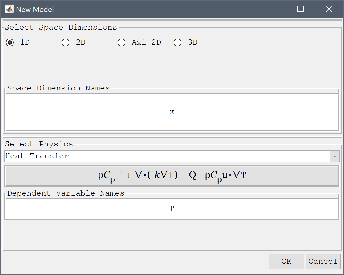
6. Press OK to finish and close the dialog box.

   
7. Switch to Grid mode by clicking on the corresponding Mode Toolbar button.

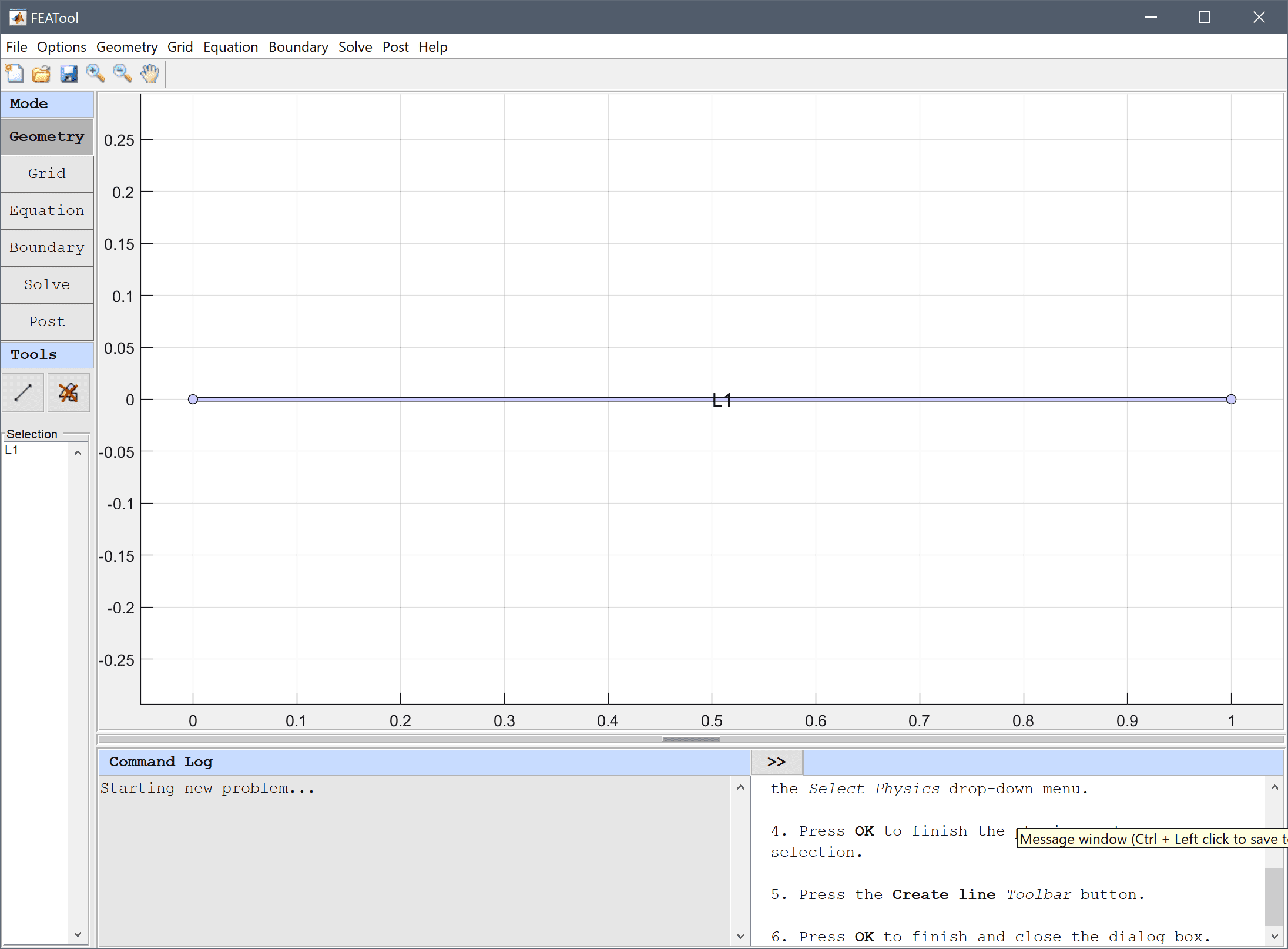
8. Press the Generate button to call the grid generation algorithm.

   
9. Switch to Equation mode by clicking on the corresponding Mode Toolbar button. (Note that the Equation Settings dialog box may look different for CFDTool.)

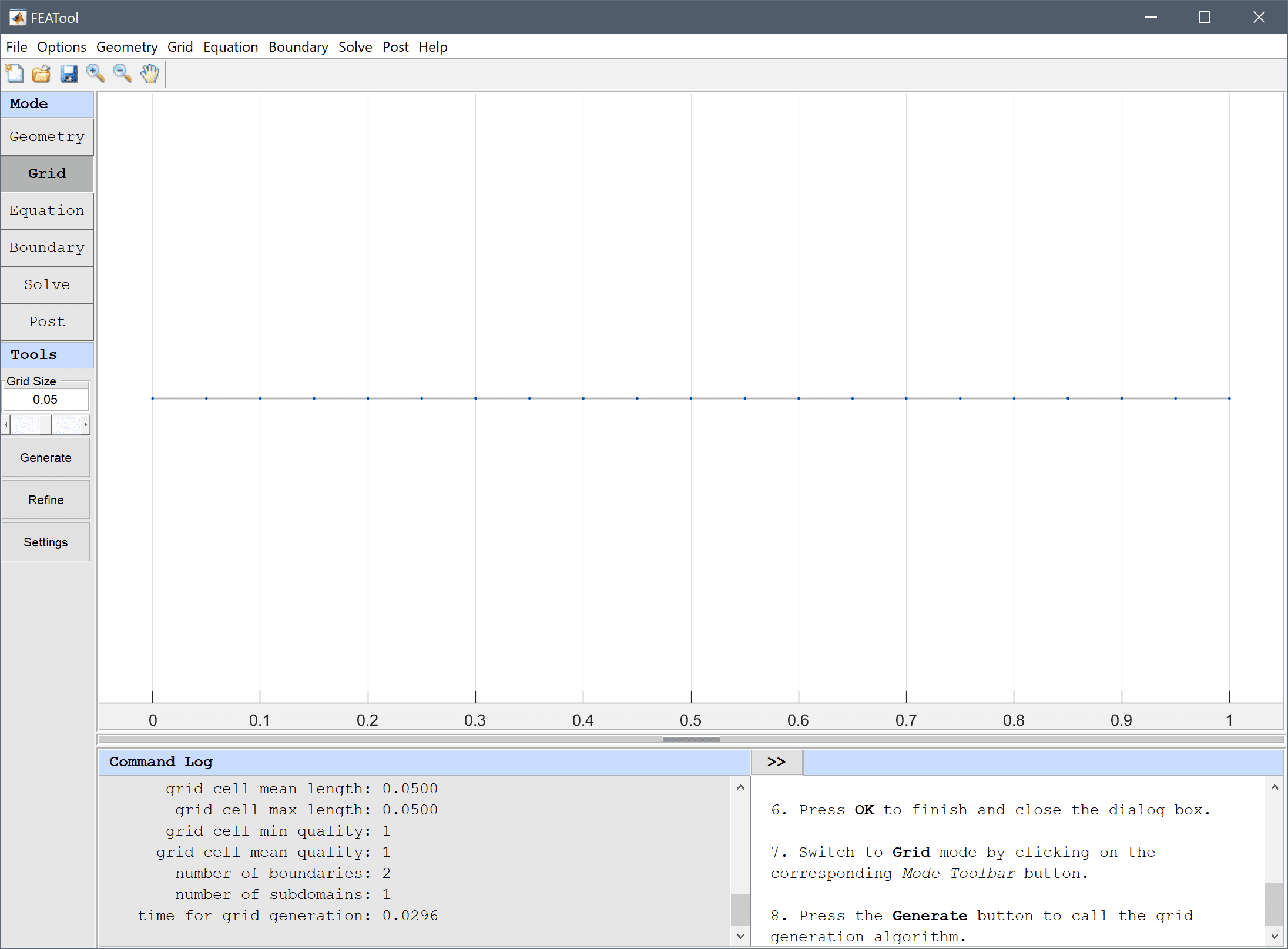
10. Enter 25 into the Initial condition for T edit field.

    
11. Press OK to finish the equation and subdomain settings specification.

A convenient way to define and store coefficients, variables, and expressions is using the Model Constants and Expressions functionality. The defined expressions can then be used in point, equation, boundary coefficients, as well as postprocessing expressions, and can easily be changed and updated in a single place. Enter an the expression for the reference temperature T_ref with two terms (n = 2).

1. Press the Constants Toolbar button.
2. Enter Tref into the edit field for the variable name.

3. Enter (24+x) + 8/pi^2*cos(pi/2*x)*exp(-pi^2/4*t) + 8/9/pi^2*cos(3*pi/2*x)*exp(-(9/4*pi^2)*t) into the edit field for the expression.

   
4. Press OK to finish and close the dialog box.
5. Switch to Boundary mode by clicking on the corresponding Mode Toolbar button.
6. Select 1 in the Boundaries list box.
7. Select Heat flux from the Heat Transfer drop-down menu.

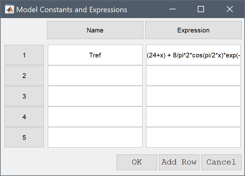
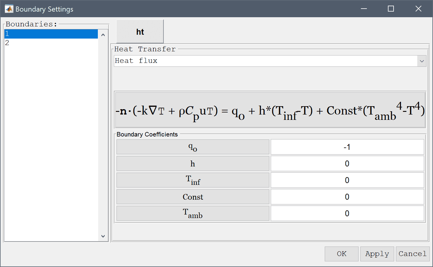
8. Enter -1 into the Inward heat flux edit field.

   
9. Select 2 in the Boundaries list box.
10. Select Temperature from the Heat Transfer drop-down menu.

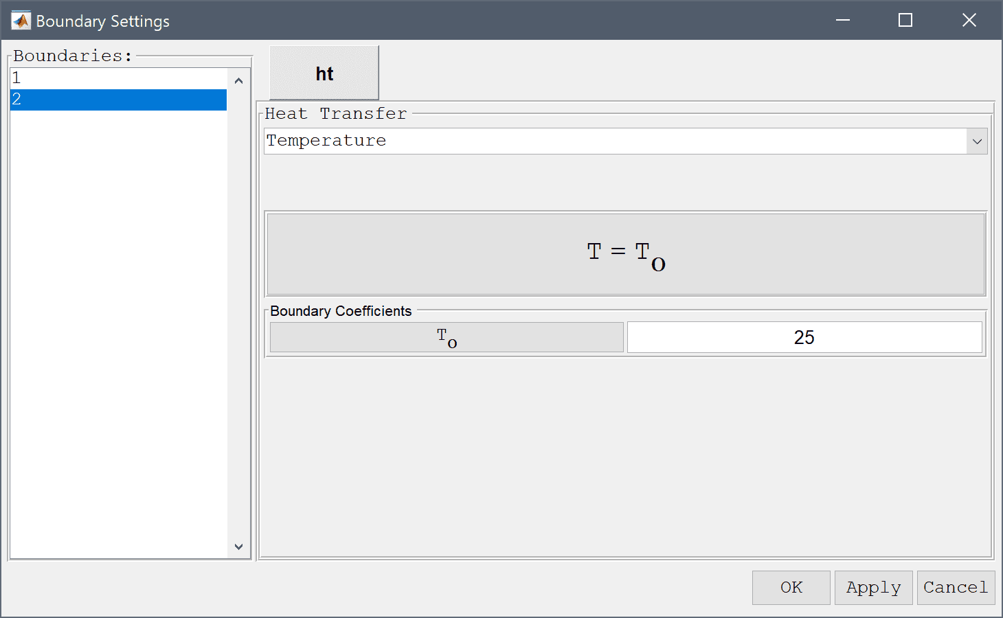
11. Enter 25 into the Temperature edit field.

    
12. Press OK to finish the boundary condition specification.
13. Switch to Solve mode by clicking on the corresponding Mode Toolbar button.
14. Press the Settings Toolbar button.
15. Select Time-Dependent from the Solution and solver type drop-down menu.
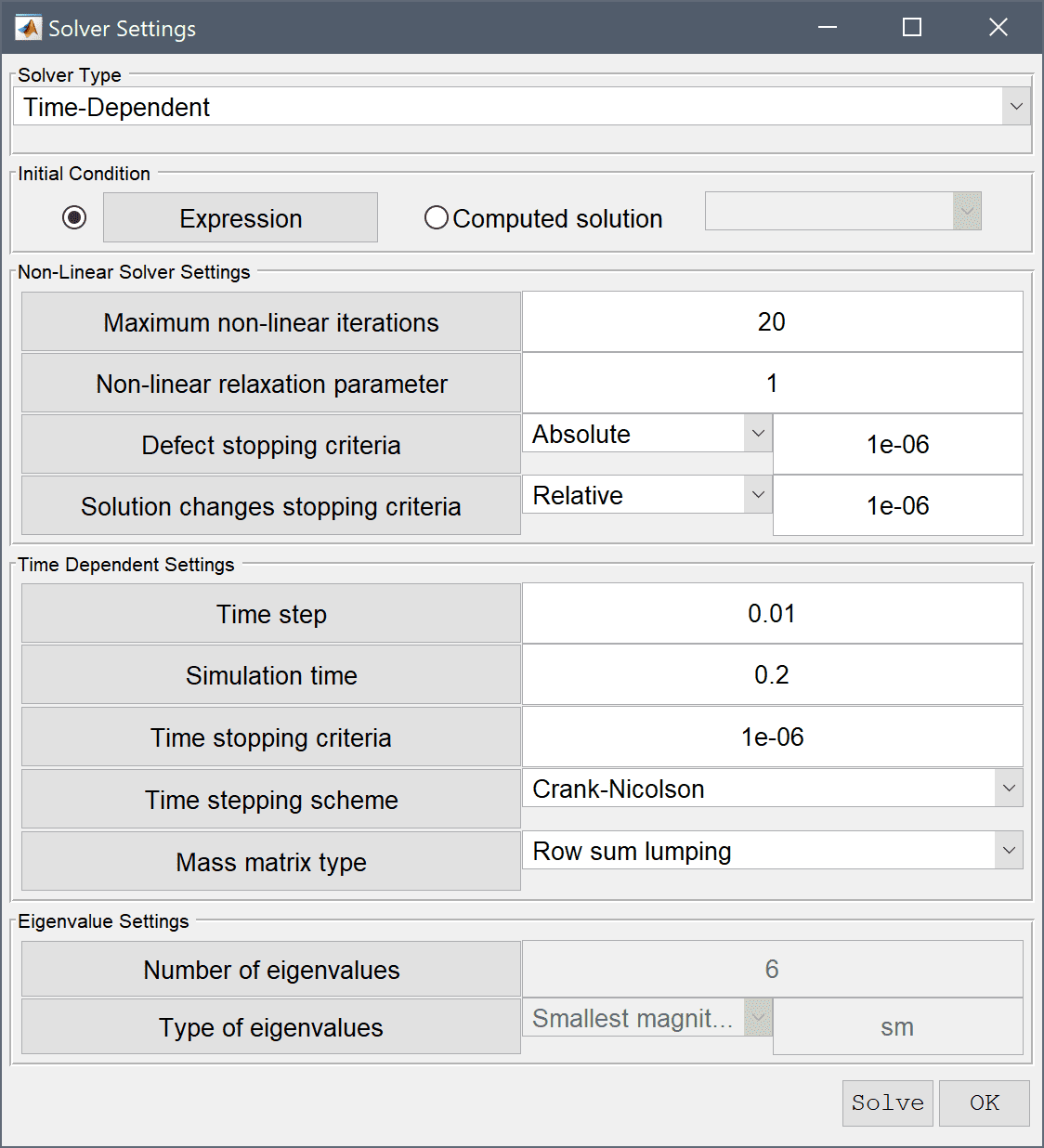
16. Enter 0.01 into the Time step size edit field.

17. Enter 0.2 into the Duration of time-dependent simulation (maximum time) edit field.

    

18. Press the Solve button.

    
19. Press the Plot Options Toolbar button.

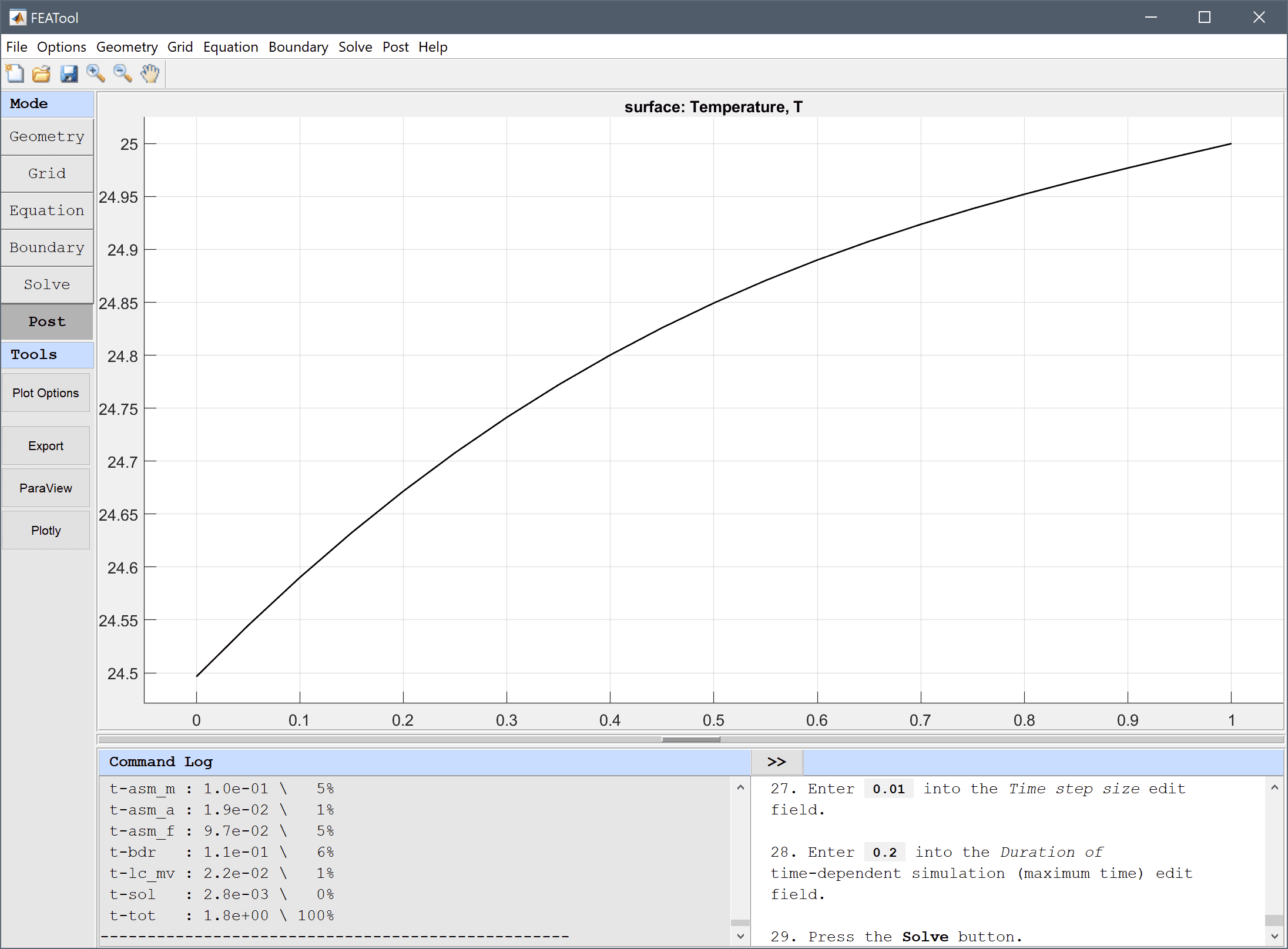
The temperature at the final time is shown where one can see that the temperature is a constant 25 degrees at the right end and is losing heat towards the left.

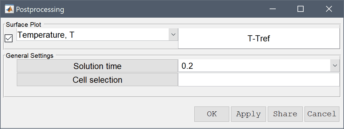
Plot and visualize the difference between the computed and reference temperature fields.

1. Enter T-Tref into the User defined surface plot expression edit field.

   
2. Press OK to plot and visualize the selected postprocessing options.
3. Select Axis/Grid Settings... from the Options menu.
4. Select the Axis equal radio button.
5. Clear the Bounding box check box.
6. Select the Axis limits radio button.

7. Enter 0 1 -1e-3 1e-3 into the Manual axis settings [xmin xmax ymin ymax] edit field.

   

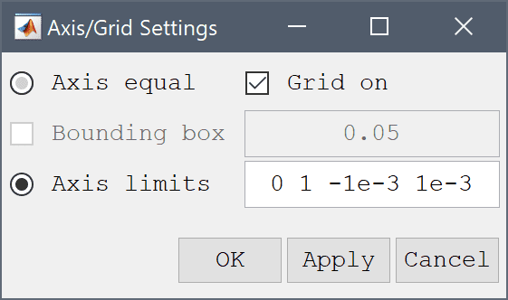
8. Press OK to finish and close the dialog box.

   

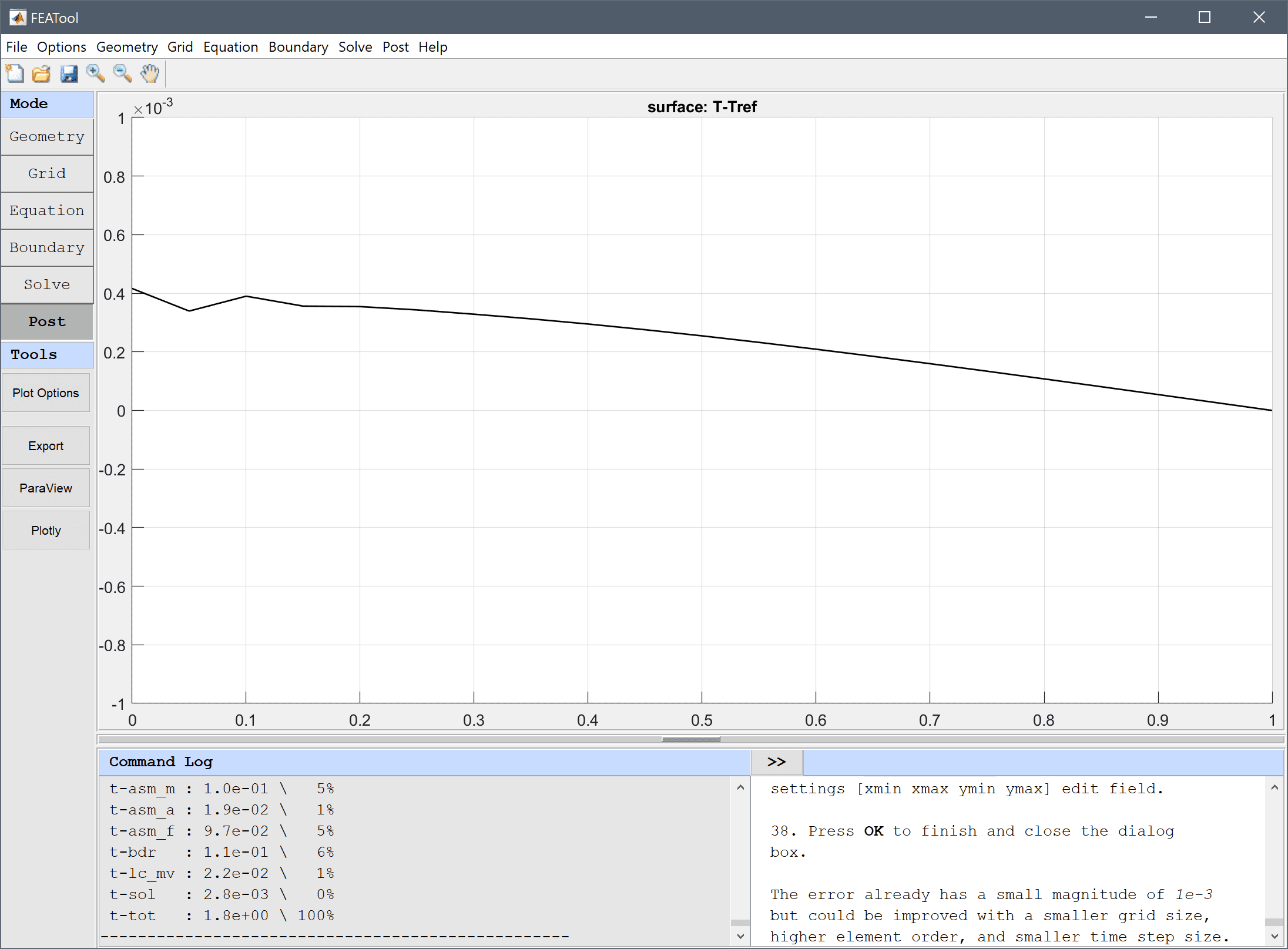
The error already has a small magnitude of 10^-3 but could be improved with a smaller grid size, higher element order, and smaller time step size.

The transient heat diffusion in a rod heat transfer model has now been completed and can be saved as a binary (.fea) model file, or exported as a programmable MATLAB m-script text file (available as the example ex_heattransfer7 script file), or GUI script (.fes) file.