|
|
FEATool Multiphysics
v1.18.0
Finite Element Analysis Toolbox
|
|
|
FEATool Multiphysics
v1.18.0
Finite Element Analysis Toolbox
|
Model of an electrostatic spherical capacitor. The example makes use of a 2D axisymmetric approximation with three subdomains, where an electric charge is applied between the middle insulating layer. For this configuration the analytic capacitance can be calculated as 4*πεrε0/dr, where dr is the thickness of the insulating layer.
This model is available as an automated tutorial by selecting Model Examples and Tutorials... > Electromagnetics > Spherical Capacitor from the File menu. Or alternatively, follow the step-by-step instructions below.
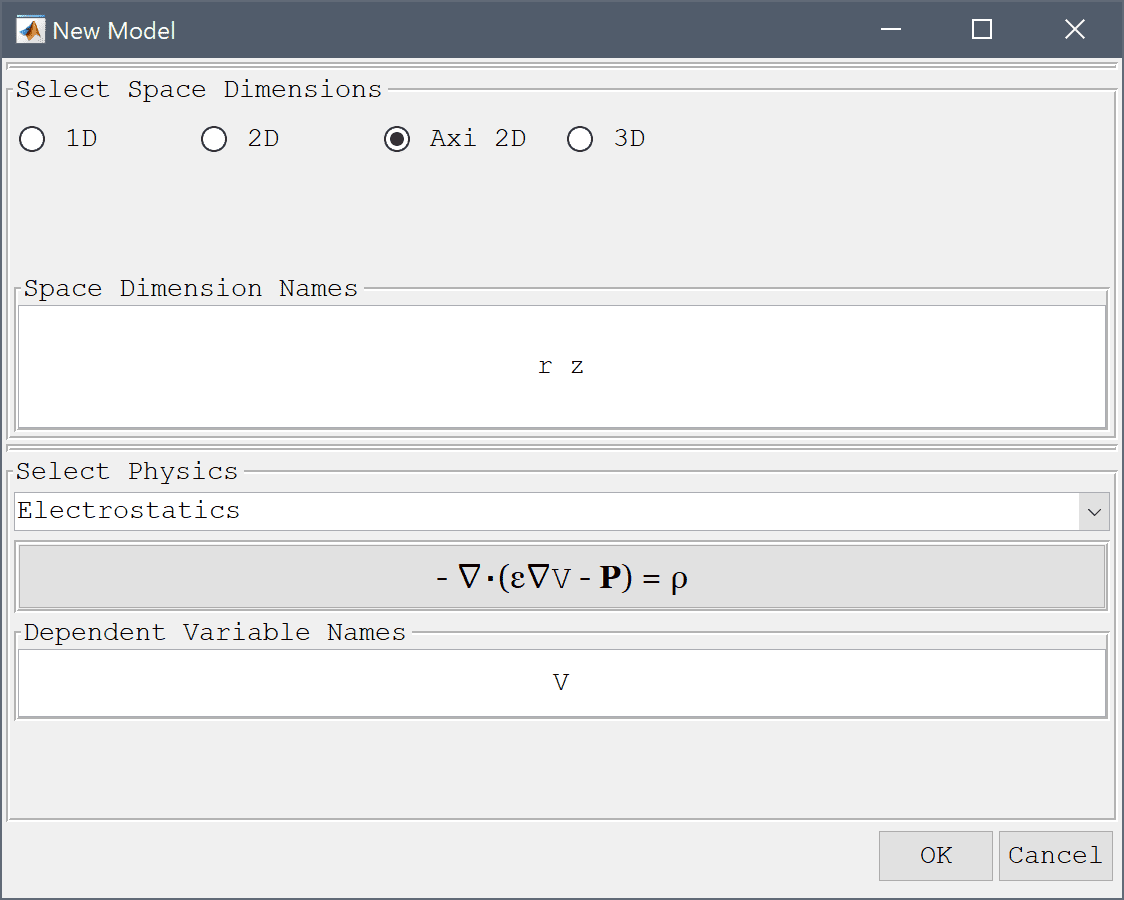
Select the Electrostatics physics mode from the Select Physics drop-down menu.
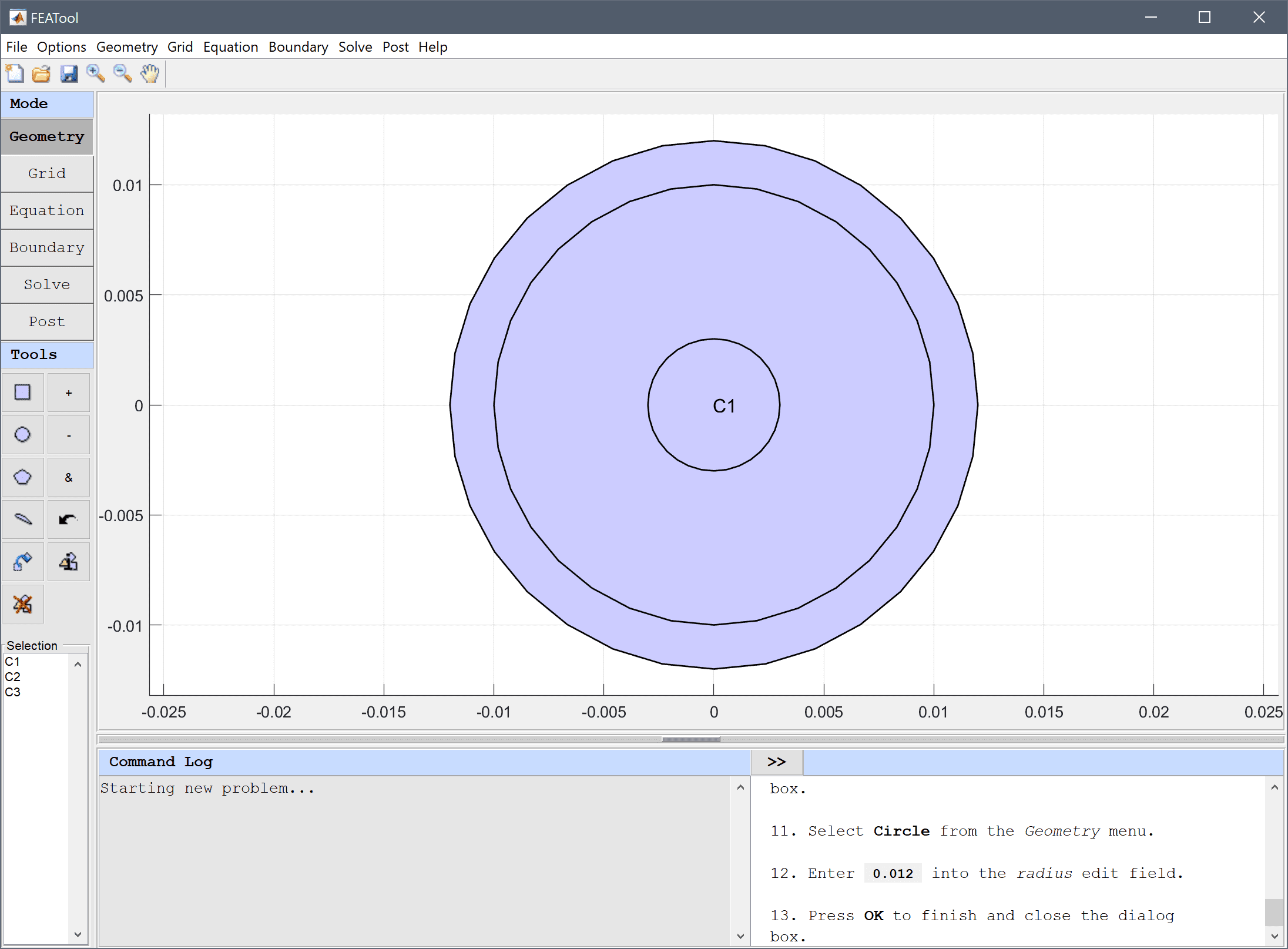
Start by creating three circles all centered at (0, 0) with radius 0.003, 0.01, and 0.012, respectively.
0.003 into the radius edit field.0.01 into the radius edit field.0.012 into the radius edit field.Press OK to finish and close the dialog box.
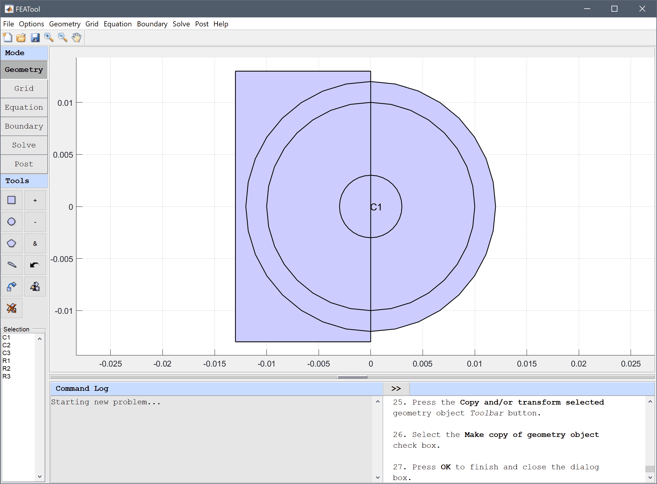
Create three rectangles on the left side of the symmetry axis (r<0) so that they cover the left side of the circles (extending a somewhat above, below and to the left).
-0.013 into the xmin edit field.0 into the xmax edit field.-0.013 into the ymin edit field.0.013 into the ymax edit field.Press OK to finish and close the dialog box.
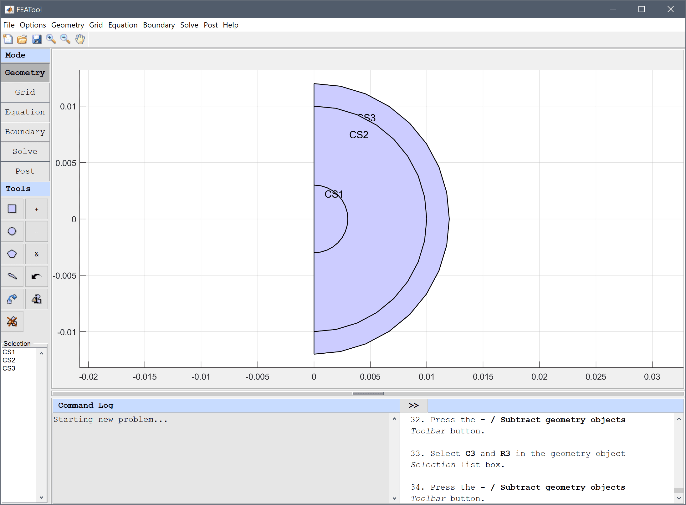
One by one subtract the rectangles from the corresponding circles so that only half circles on right side half plane remain.
C1 - R1 into the Geometry Formula edit field.Press the - / Subtract geometry objects Toolbar button.
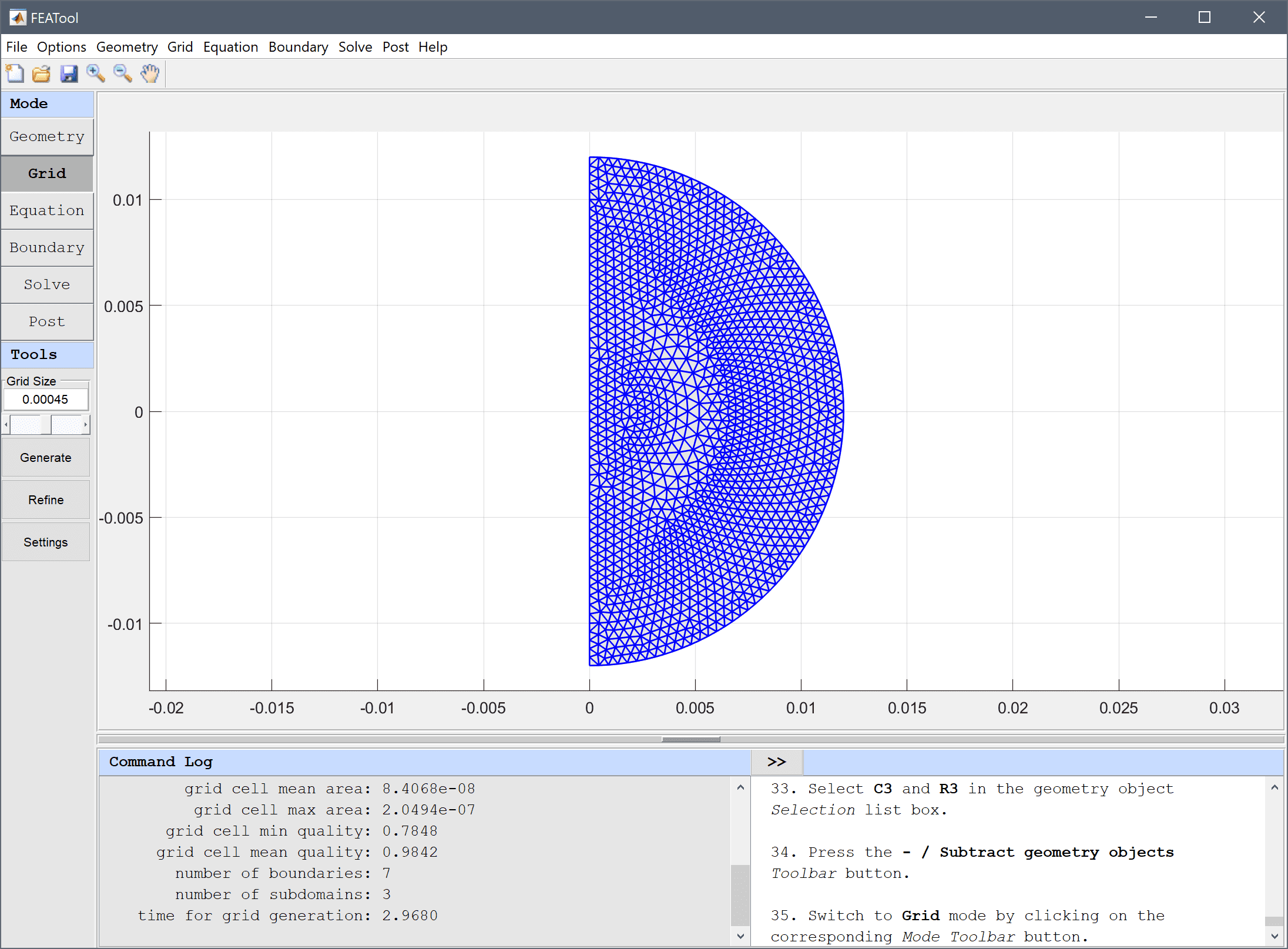
Switch to Grid mode by clicking on the corresponding Mode Toolbar button.
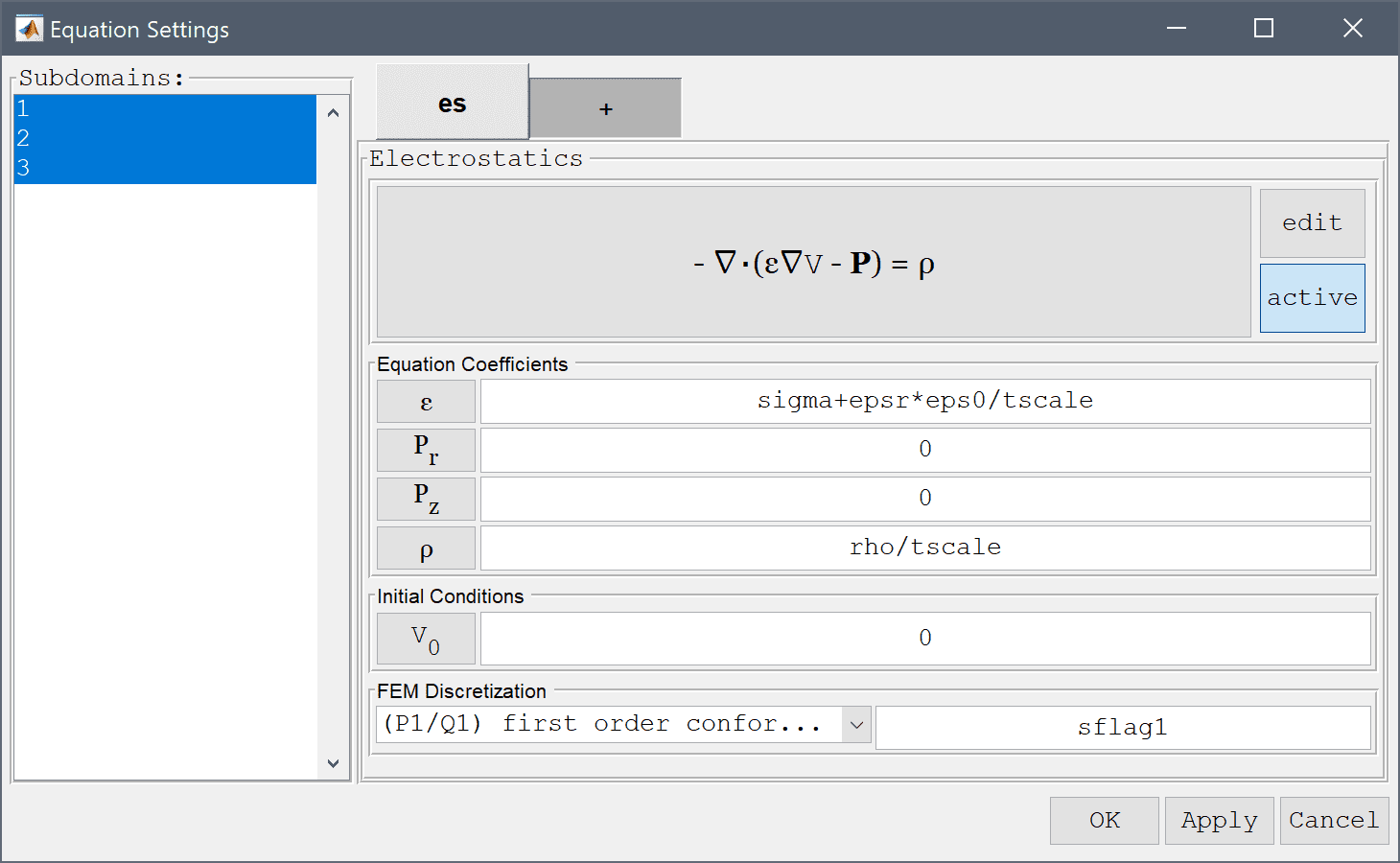
Press the Equation mode button to switch from grid mode to physics and equation/subdomain specification mode. In the Equation Settings dialog box that automatically opens, select all Subdomains (1-3) and enter sigma+epsr*eps0/tscale for the Permittivity, ε, and rho/tscale for the Space charge density, ρ.
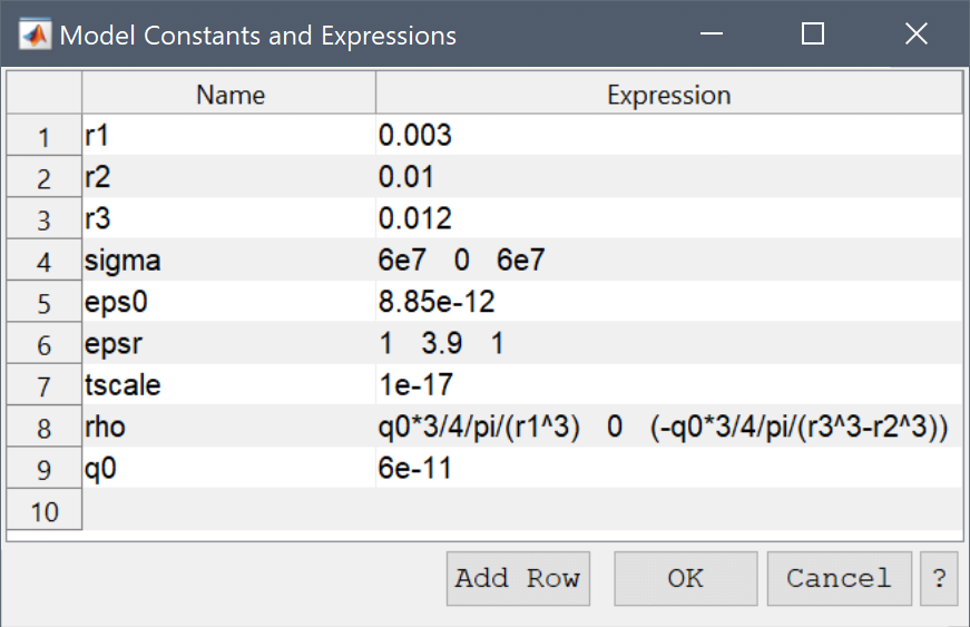
| Name | Expression |
|---|---|
| r1 | 0.003 |
| r2 | 0.01 |
| r3 | 0.012 |
| sigma | 6e7 0 6e7 |
| eps0 | 8.85e-12 |
| epsr | 1 3.9 1 |
| tscale | 1e-17 |
| rho | q0*3/4/pi/(r1^3) 0 -q0*3/4/pi/(r3^3-r2^3) |
| q0 | 6e-11 |
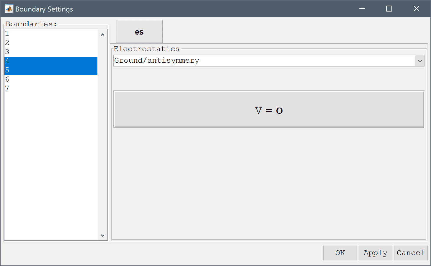
Select the left symmetry boundaries, 1-3, and 6-7 in the Boundaries list box, and select the Insulation/symmetry boundary condition from the Electrostatics drop-down menu.
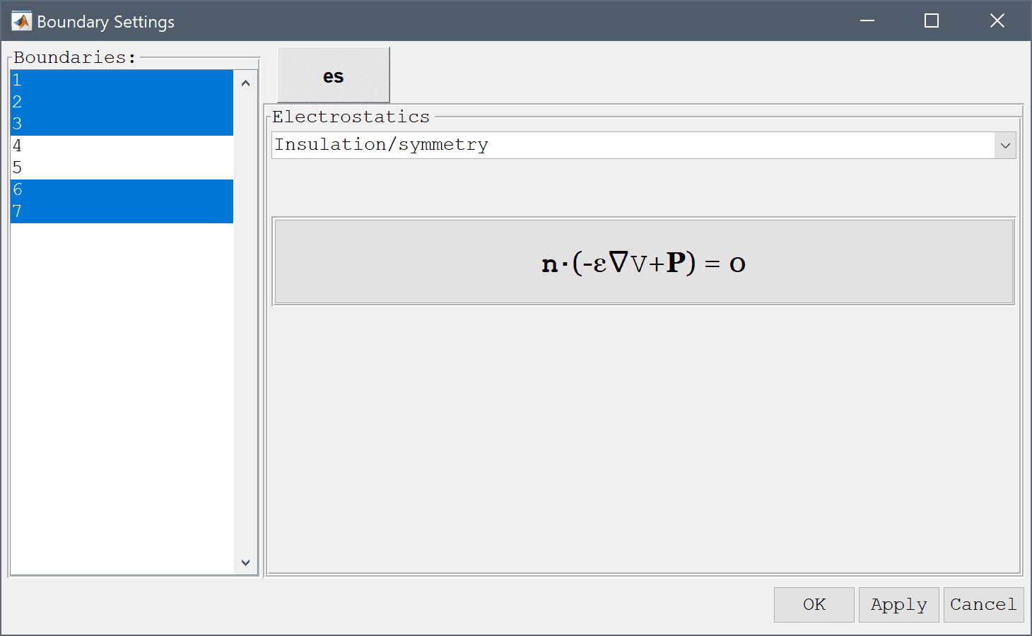
Then select the outer boundaries, 4 and 5 in the Boundaries list box, and set them to Ground/antisymmetry (from the Electrostatics drop-down menu).
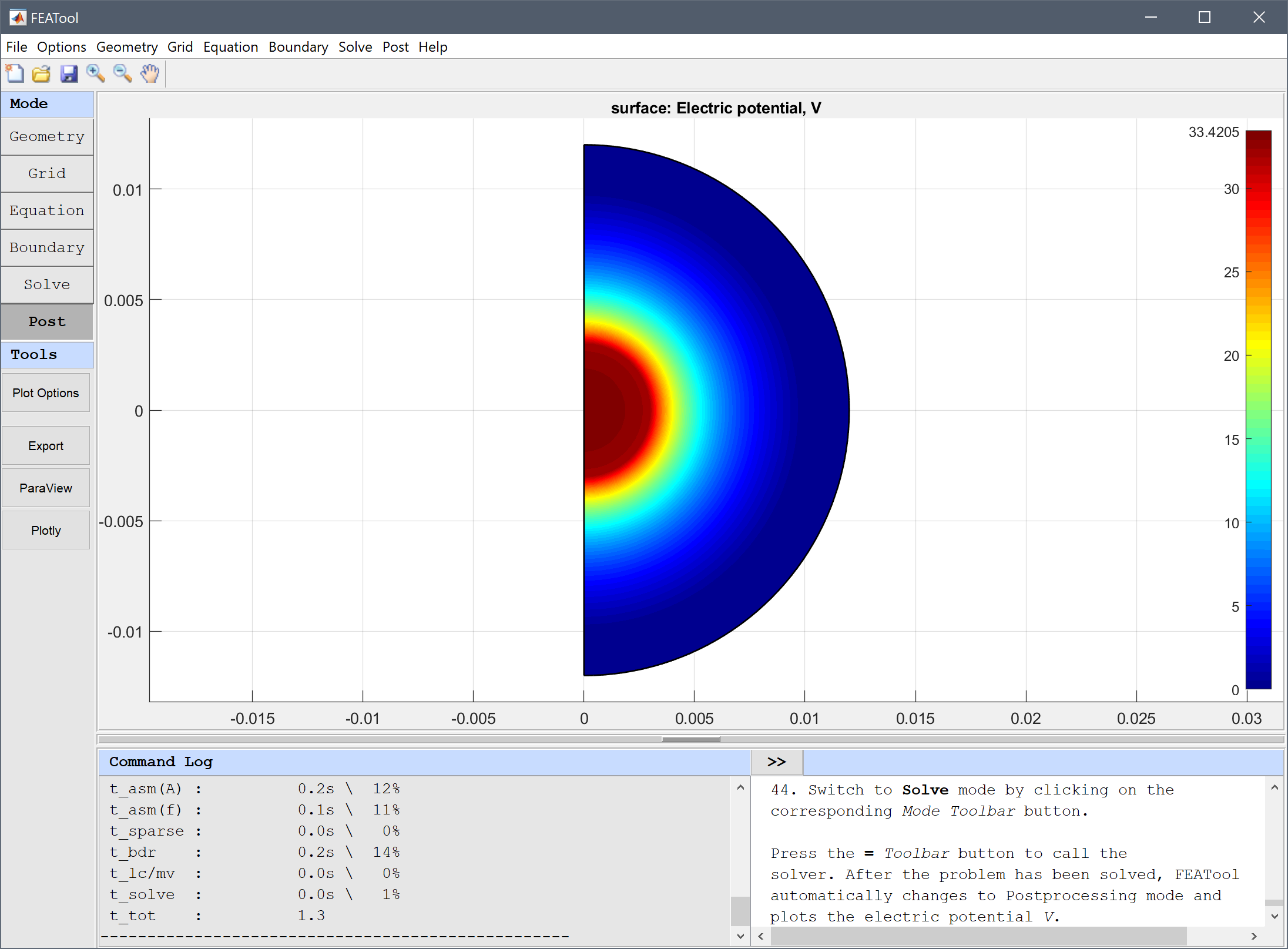
Switch to Solve mode by clicking on the corresponding Mode Toolbar button, and press the = Toolbar button to call the solver. After the problem has been solved, FEATool automatically changes to Postprocessing mode and plots the electric potential V.
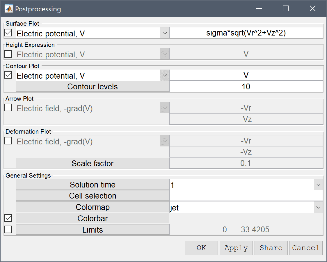
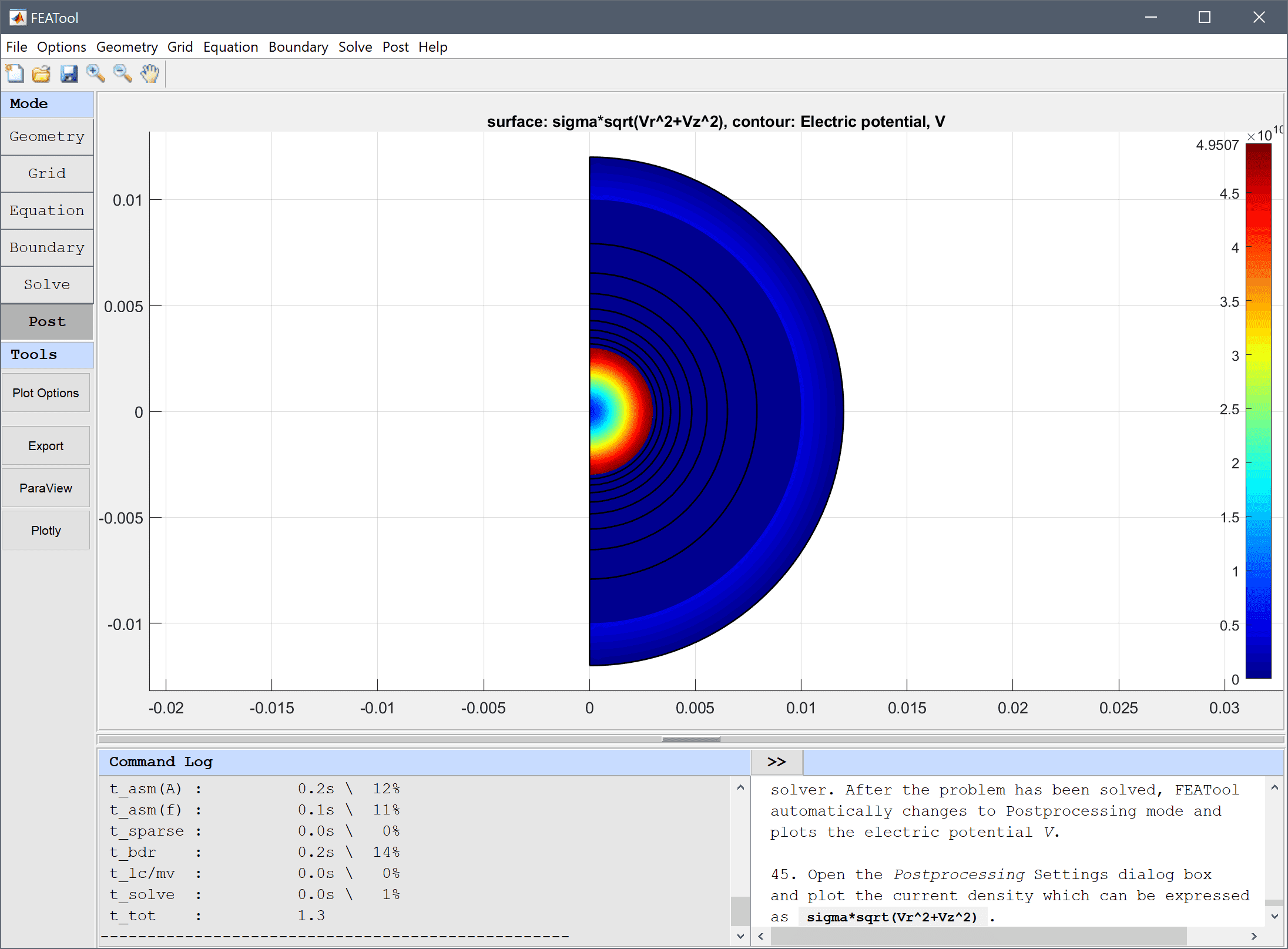
Open the Postprocessing Settings dialog box and plot the current density which can be expressed as sigma*sqrt(Vr^2+Vz^2)
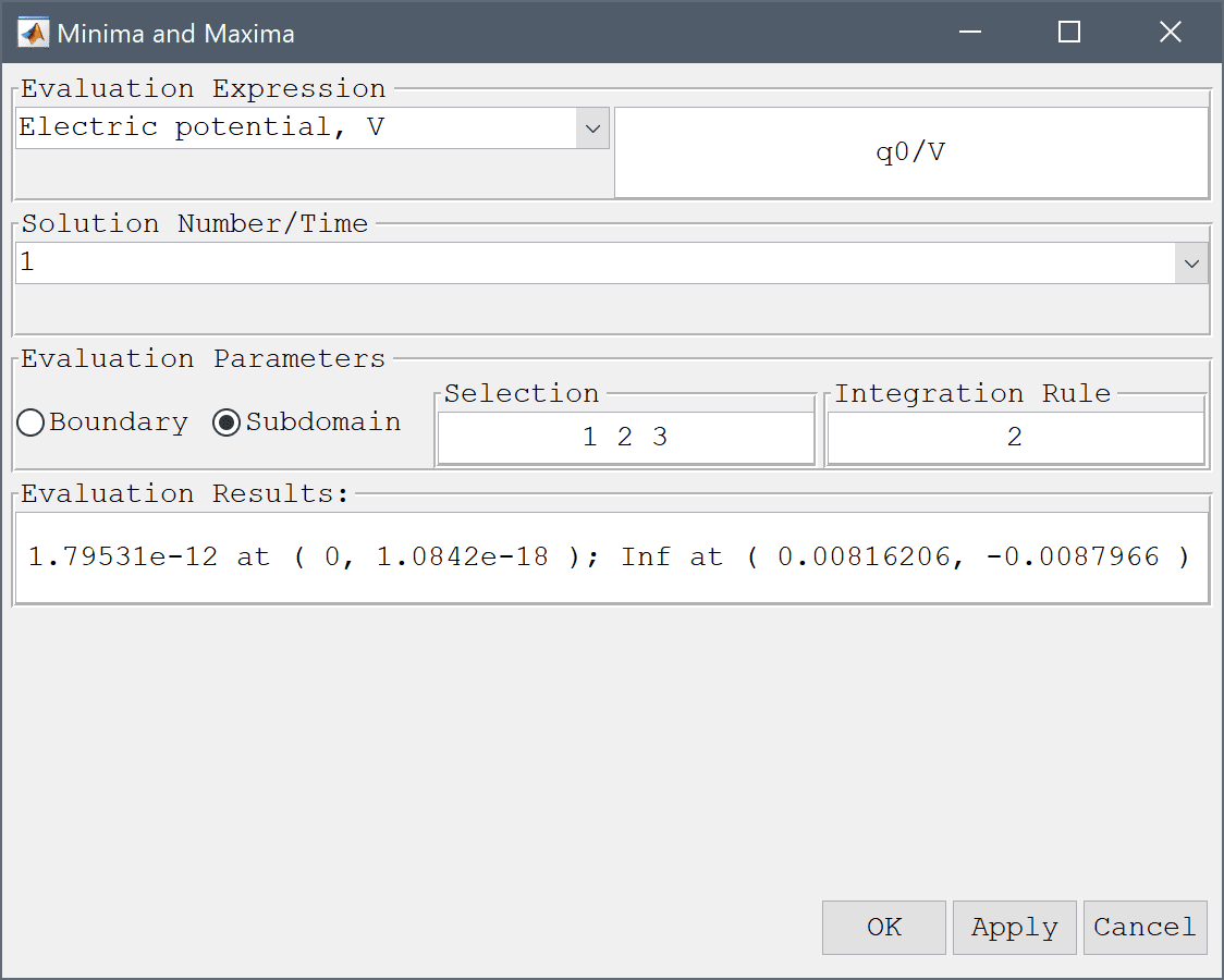
To verify the solution, one can calculate the capacitance as q0/( Vmax - Vmin ) where Vmax can be found by using the Min/Max Evaluation... option from the Post menu (Vmin will be 0).
q0/V into the edit field.Press the Apply button.
Alternatively, one can integrate the expression for the energy E = ε0εr(Vr2+Vz2)πr over all subdomains, where the capacitance then can be calculated as q02/(2·E).
Compare the computed capacitances with the analytical expression 4*πεrε0/( 1/0.003 - 1/0.01 ) which in this example should be equal to 1.8588e-12.
The spherical capacitor electromagnetics model has now been completed and can be saved as a binary (.fea) model file, or exported as a programmable MATLAB m-script text file (available as the example ex_electrostatics2 script file), or GUI script (.fes) file.
To visualize the full 3D solution from the axisymmetic model, the data can be exported and processed on the MATLAB command line interface (CLI) console with the Export Model Data Struct to MATLAB option from the File menu. The postrevolve and postplot functions can then be applied to revolve and visualize the data, for example
fea_revolved = postrevolve( fea, 24, 0.75 );

postplot( fea_revolved, 'surfexpr', 'V', ...
          'parent', figure, 'axis', 'off', 'colorbar', 'off' )
view(70, 25)