Magnetic Field Around a Horseshoe Magnet

Example of simulation and visualization of the two-dimensional static magnetic potential field around a u-shaped permanent magnet.

Tutorial

This model is available as an automated tutorial by selecting Model Examples and Tutorials... > Electromagnetics > Magnetic Field Around a Permanent Magnet from the File menu. Or alternatively, follow the step-by-step instructions below.

1. To start a new model click the New Model toolbar button, or select New Model... from the File menu.

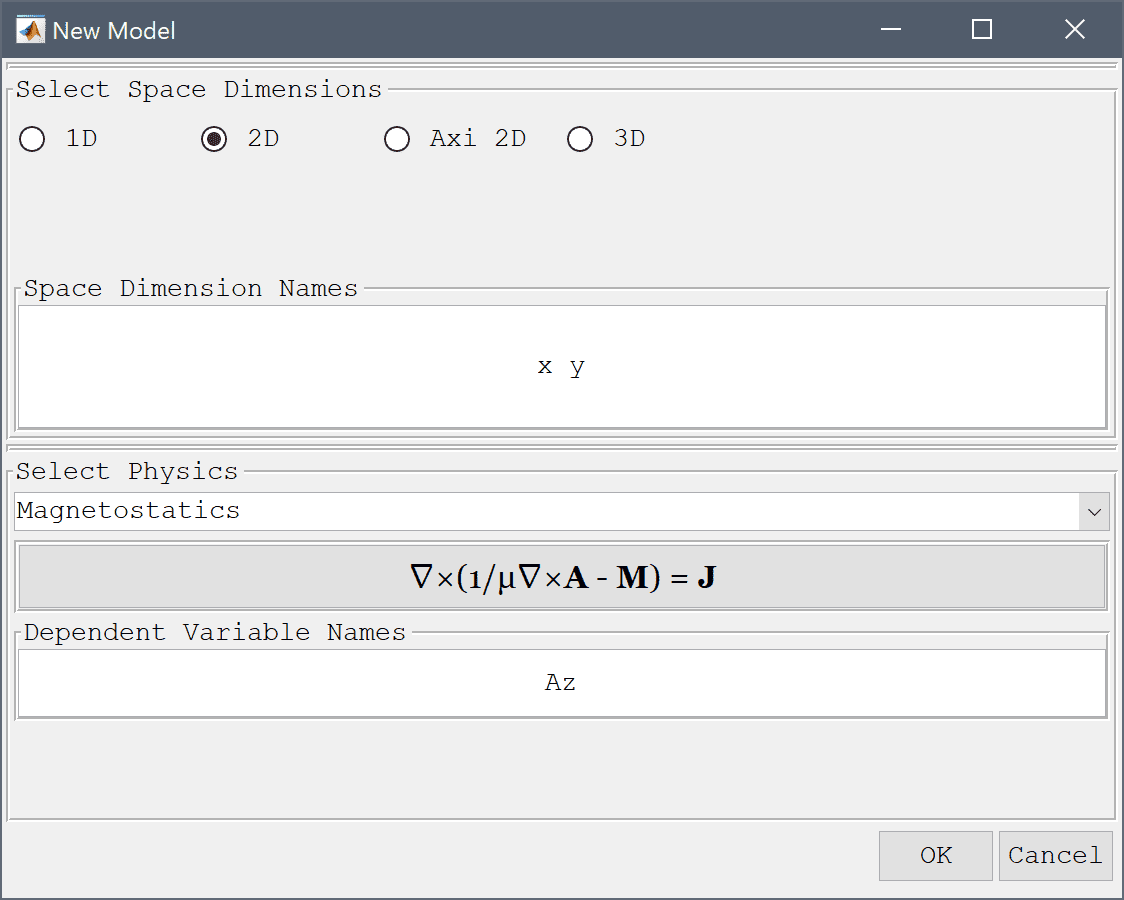
2. Select the Magnetostatics physics mode from the Select Physics drop-down menu.

   
3. Press OK to finish the physics mode selection.

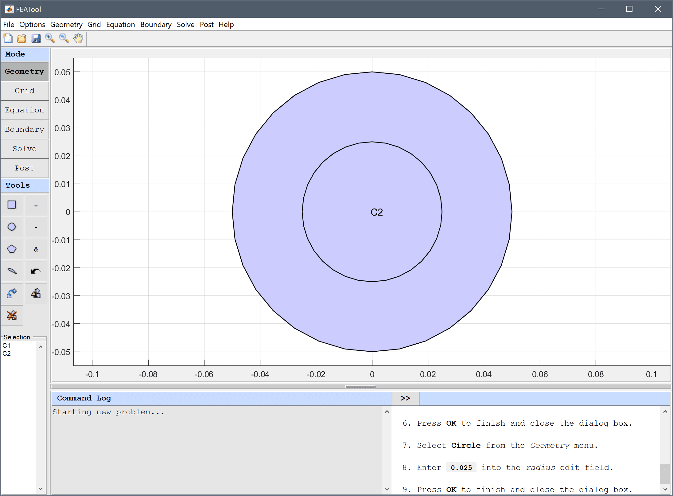
Start by creating two circles centered at (0, 0) and with radius 0.05, and 0.0025, respectively.

1. Select Circle from the Geometry menu.
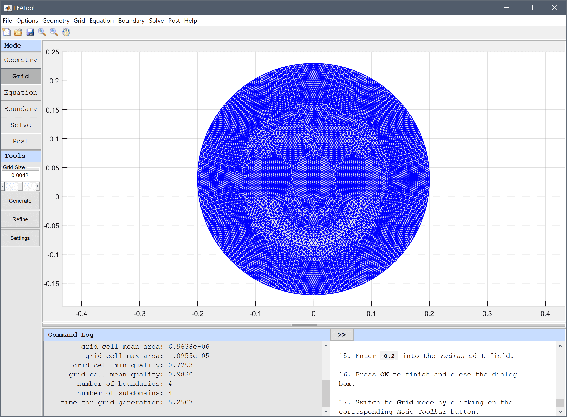
2. Enter 0.05 into the radius edit field.
3. Press OK to finish and close the dialog box.
4. Select Circle from the Geometry menu.
5. Enter 0.025 into the radius edit field.

6. Press OK to finish and close the dialog box.

   
7. Create three rectangles with dimensions according to the table below

x_min	x_max	y_min	y_max
-0.06	-0.05	0.025	-0.15
0.06	-0.025	0.05	0.15
0	0	0	-0.2
0.06	0.06	0.06	0.2

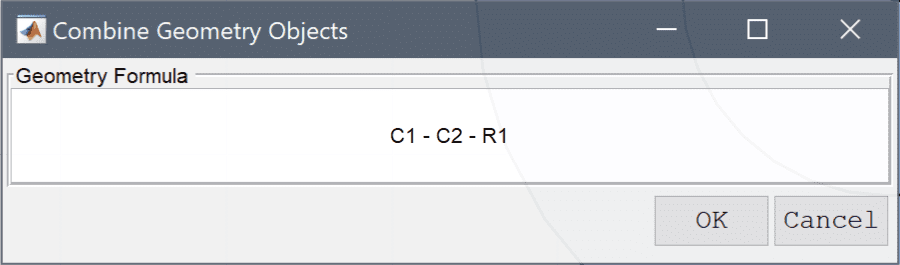
1. Subtract rectangle R1 and the smaller circle C2 from C1 using the formula C1 - C2 - R1 in the Combine Objects... option of the Geometry menu.

   
2. Press OK to finish and close the dialog box.

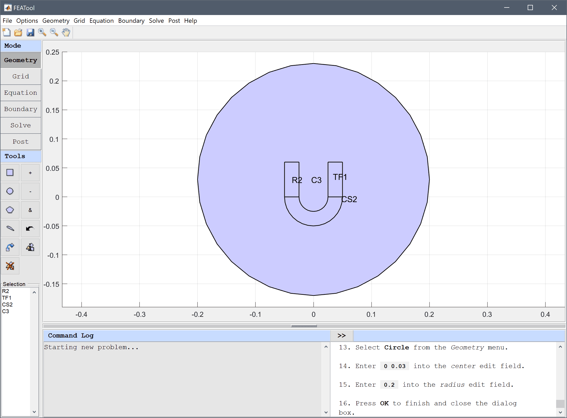
Lastly, create a larger circle for the surrounding domain.

1. Select Circle from the Geometry menu.
2. Enter 0 0.03 into the center edit field.
3. Enter 0.2 into the radius edit field.

4. Press OK to finish and close the dialog box.

   

5. Switch to Grid mode by clicking on the corresponding Mode Toolbar button.

   

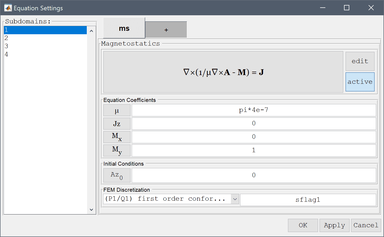
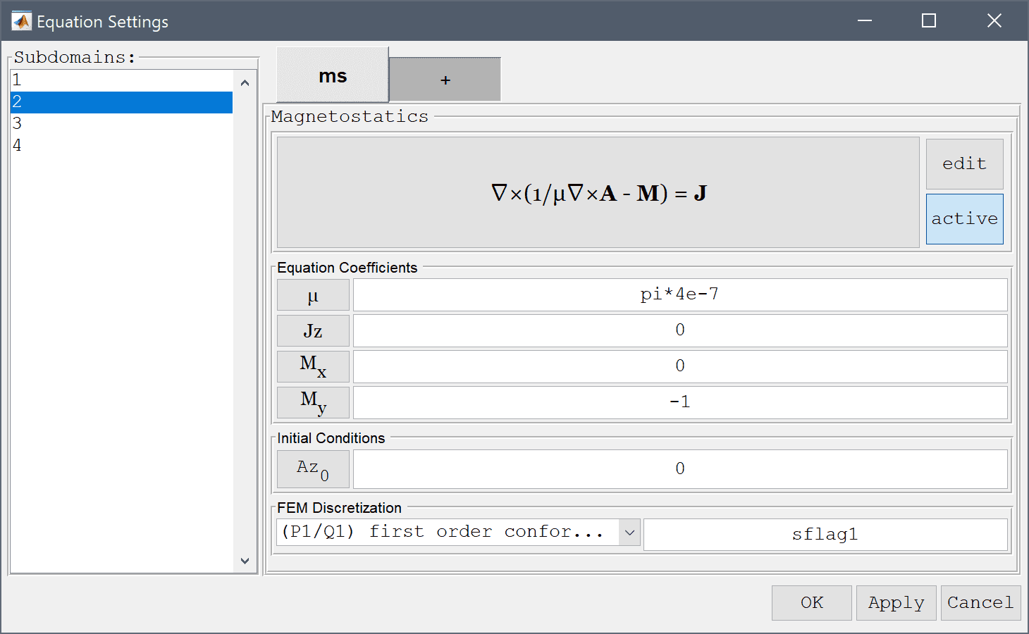
6. Press the Equation mode button to switch from grid mode to physics and equation/subdomain specification mode. In the Equation Settings dialog box that automatically opens, prescribe opposing magnetization of the magnet ends by setting the Magnetization, My coefficient to 1 and -1 in subdomains 1 and 2, respectively. Leave the magnet curve and outer domain with zero magnetization.

   
   
7. Switch to Boundary mode by clicking on the corresponding Mode Toolbar button.

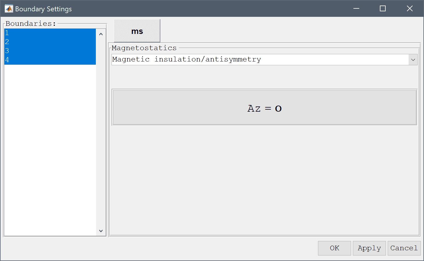
In Boundary mode, set or leave all the boundary conditions to the default Magnetic insulation/antisymmetry selection.

1. Now that the problem is fully specified, press the Solve Mode Toolbar button to switch to solve mode. Then press the = Tool button to call the solver with the default solver settings.
2. Switch to Solve mode by clicking on the corresponding Mode Toolbar button.

3. After the problem has been solved, FEATool automatically changes to Postprocessing mode and plots the Magnetic potential, Az. Contours and arrow plots of the magnetic field can be selected by using the Postprocessing Settings dialog box.

   
   

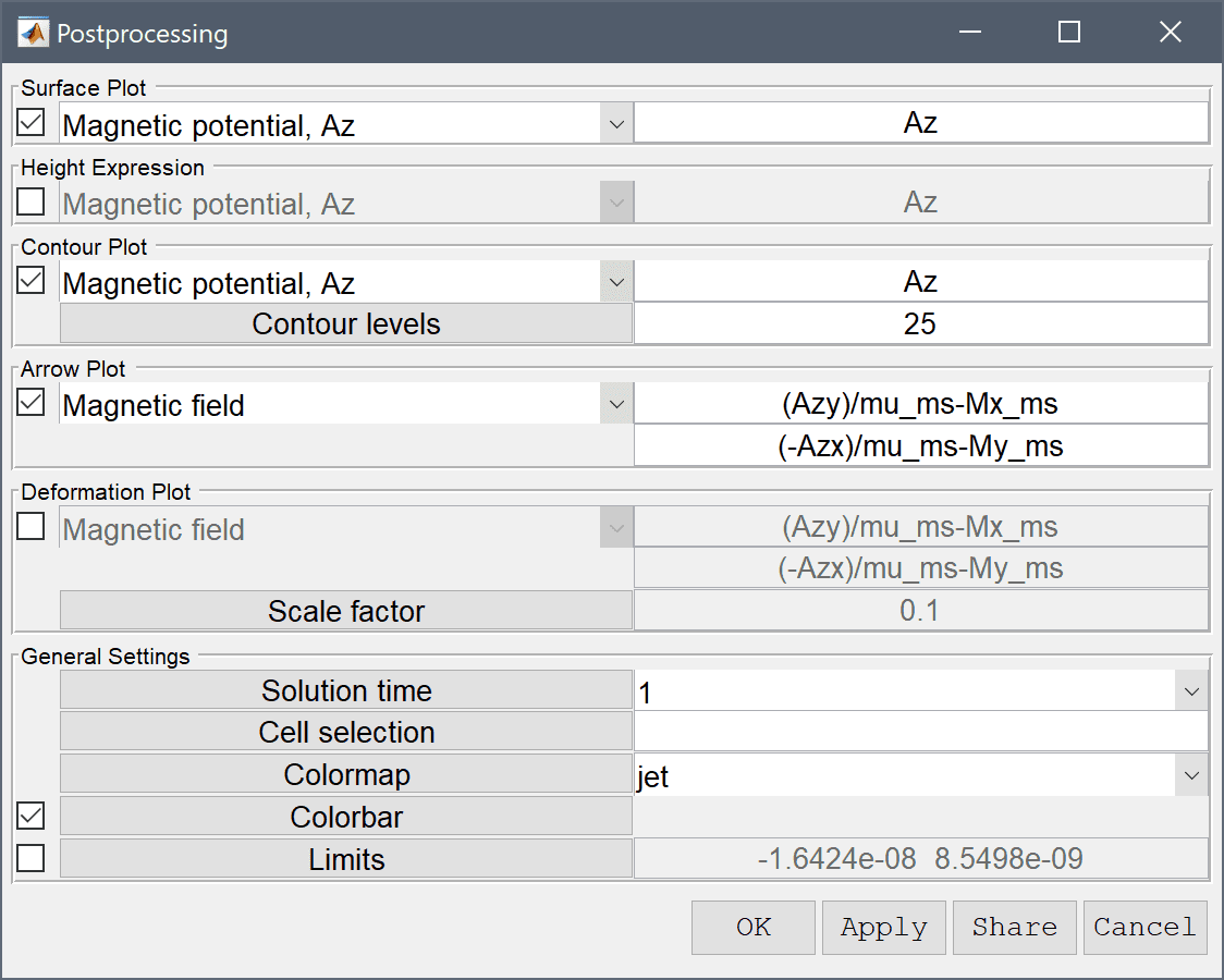
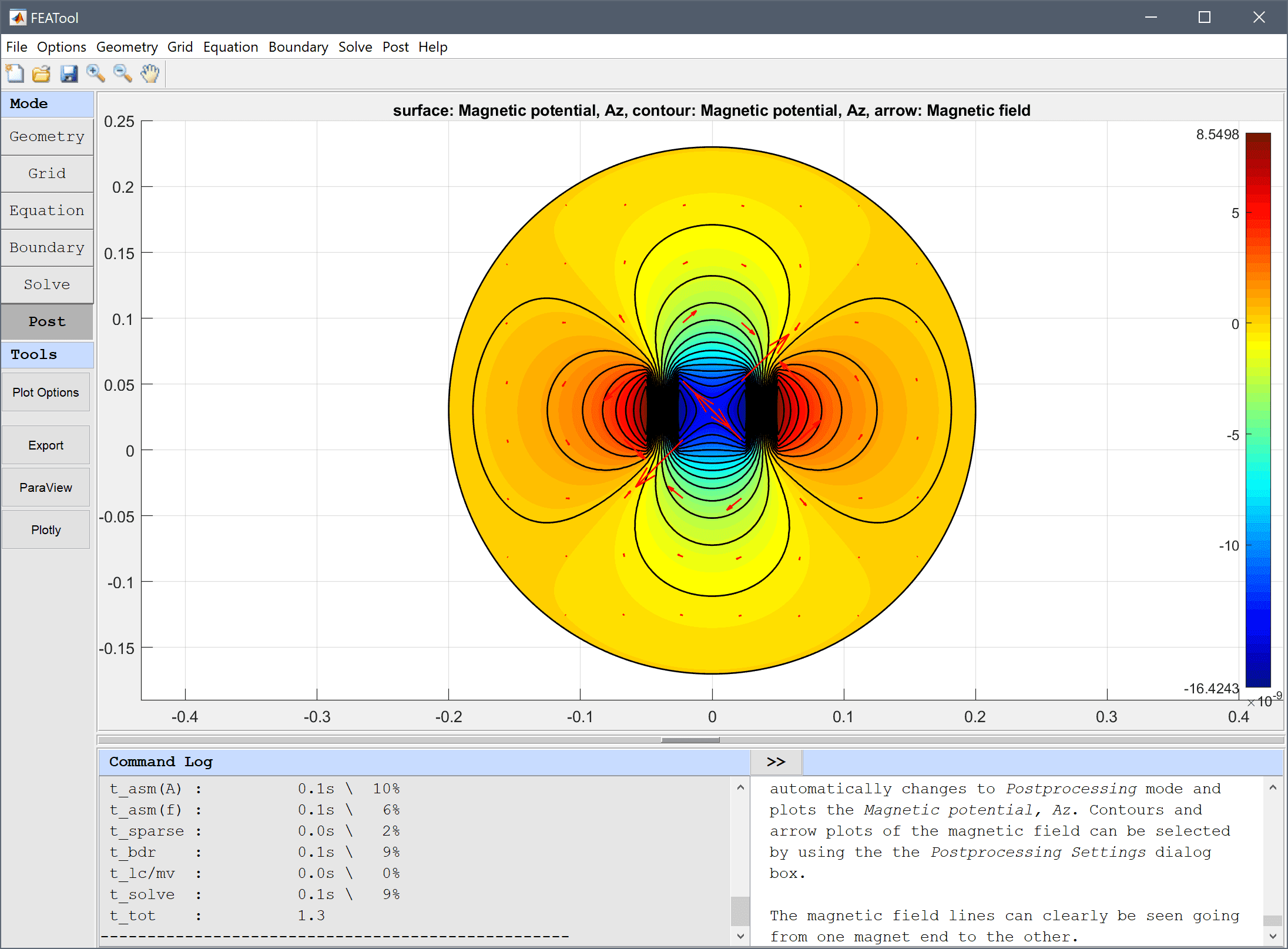
The magnetic field lines can clearly be seen going from one magnet end to the other.

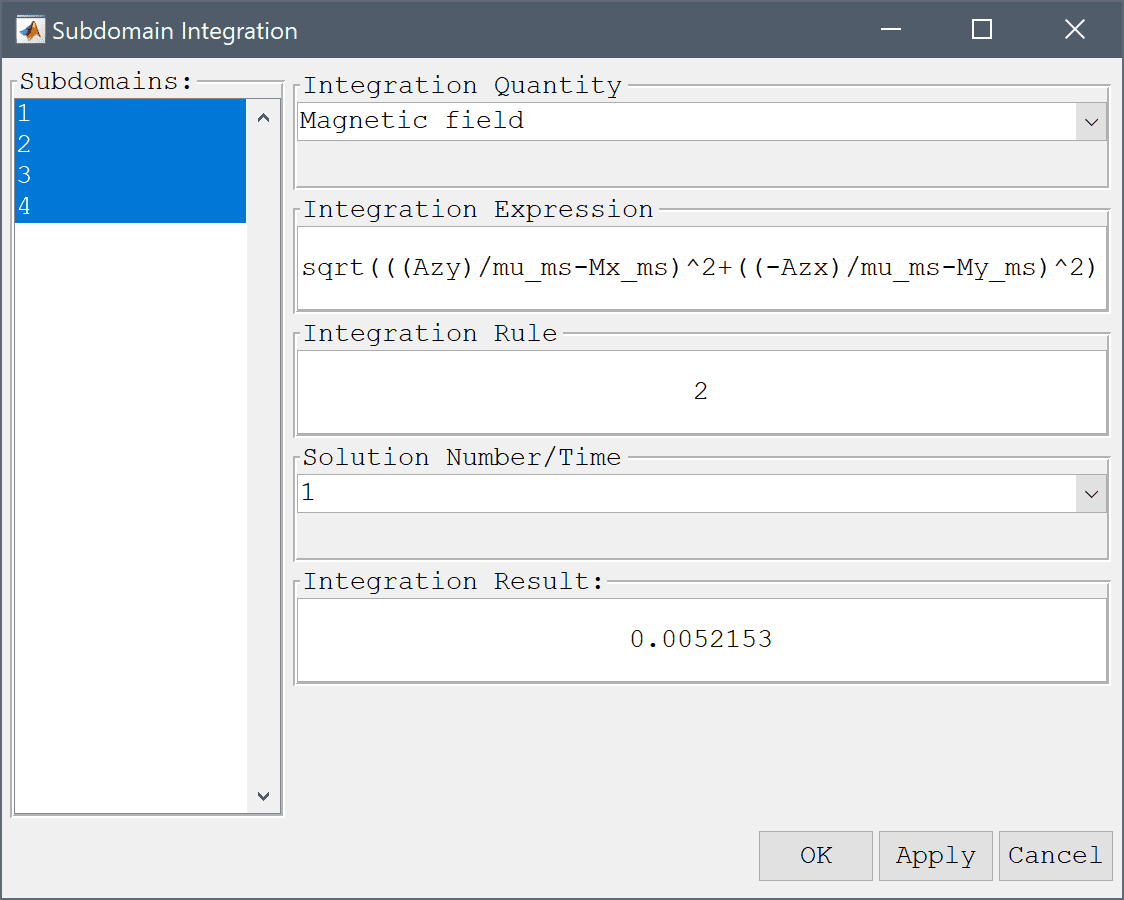
1. To verify the solution, choose the Subdomain Integration... option in the Post menu, and integrate the Magnetic potential, Az and Magnetic field over all subdomains, the integrals should result in values around -7.1e-11 and 0.005, respectively.

   

The magnetic field around a permanent magnet electromagnetics model has now been completed and can be saved as a binary (.fea) model file, or exported as a programmable MATLAB m-script text file (available as the example ex_magnetostatics2 script file), or GUI script (.fes) file.