Two Material Wave Guide Interface

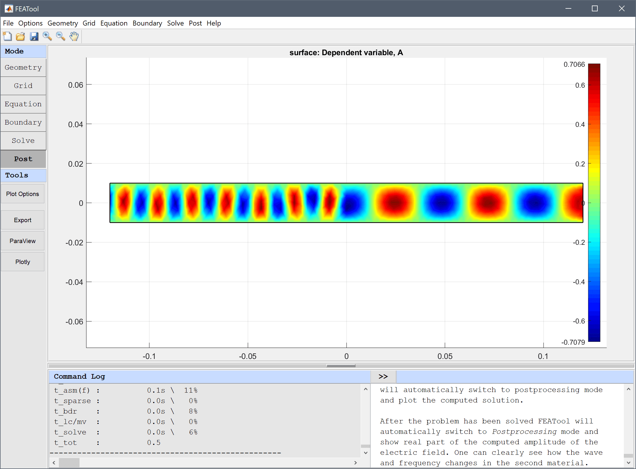
Simulation of a wave guide interface with two different materials. The changing diffraction pattern of planar time harmonic waves is investigated using the Helmholtz equation

\[ -( \frac{\partial^2 A}{\partial x^2} + \frac{\partial^2 A}{\partial y^2} ) - k^2 A = 0 \]

Tutorial

This model is available as an automated tutorial by selecting Model Examples and Tutorials... > Electromagnetics > Two Material Wave Guide Interface from the File menu. Or alternatively, follow the step-by-step instructions below.

1. To start a new model click the New Model toolbar button, or select New Model... from the File menu.
2. Select the Custom Equation physics mode from the Select Physics drop-down menu.

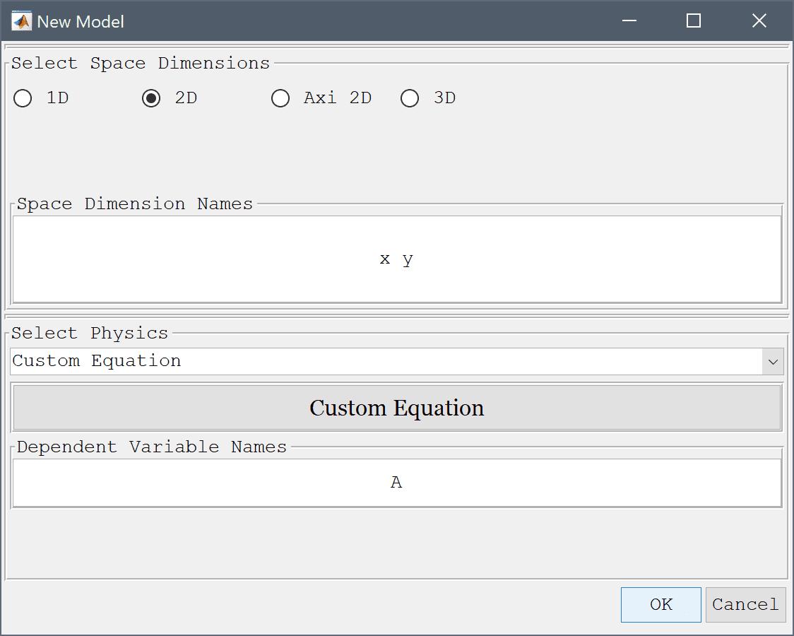
3. Enter A into the Dependent Variable Names edit field.

   
4. Press OK to finish the physics mode selection.

The geometry consists of two rectangles for the different materials.

1. Select Rectangle from the Geometry menu.
2. Enter -0.12 into the x_min edit field.
3. Enter 0 into the x_max edit field.
4. Enter -0.01 into the y_min edit field.
5. Enter 0.01 into the y_max edit field.
6. Press OK to finish and close the dialog box.
7. Select R1 in the geometry object Selection list box.
8. Press the Copy and/or transform selected geometry object Toolbar button.
9. Select the Make copy of geometry object check box.
10. Enter 0.12 0 into the Space separated string of displacement lengths edit field.
11. Press OK to finish and close the dialog box.
12. Switch to Grid mode by clicking on the corresponding Mode Toolbar button.
13. Press the Refine Toolbar button.
14. Switch to Equation mode by clicking on the corresponding Mode Toolbar button.
15. Press the edit button.

Enter the Helmholtz equation in the Edit Equations dialog box.

1. Enter -(Ax_x + Ay_y) - k^2*A_t = 0 into the Equation for A edit field.
2. Press OK to finish and close the dialog box.
3. Press OK to finish the equation and subdomain settings specification.
4. Press the Constants Toolbar button, or select the corresponding entry from the Equation menu, and add the following modeling constants for the speed of light, frequency, and wave number in the Model Constants and Expressions dialog box. Note that the wave number is scaled by a factor of two in the left subdomain (entering a space separated list allows prescribing constants on a per subdomain basis).

Name	Expression
c	3e9
f	1e11
sfac	2   1
k	sfac*2*pi*f/c

1. Switch to Boundary mode by clicking on the corresponding Mode Toolbar button.

Set homogenous Dirichlet conditions A = 0 for the absorbing walls.

An incoming planar wave is featured at the inlet with the complex boundary condition n·∇(A) + k·i·A = 2·k·i which can be implemented as a Neumann boundary condition.

1. Select boundary number 5 in the Boundaries list box.
2. Select the Neumann, g_A radio button.
3. Enter -k*i*A + 2*k*i into the Dirichlet/Neumann coefficient edit field.

The outlet is assumed non-reflective and n·∇(A) + k·i·A = 0.

1. Select number 3 in the Boundaries list box.
2. Select the Neumann, g_A radio button.
3. Enter -k*i*A into the Dirichlet/Neumann coefficient edit field.
4. Press OK to finish the boundary condition specification.
5. Switch to Solve mode by clicking on the corresponding Mode Toolbar button.
6. Press the = Toolbar button to call the solver. After the problem has been solved FEATool will automatically switch to postprocessing mode and plot the computed solution.

After the problem has been solved FEATool will automatically switch to Postprocessing mode and show real part of the computed amplitude of the electric field. One can clearly see how the wave and frequency changes in the second material.

The two material wave guide interface electromagnetics model has now been completed and can be saved as a binary (.fea) model file, or exported as a programmable MATLAB m-script text file, or GUI script (.fes) file.