|
|
FEATool Multiphysics
v1.18.1
Finite Element Analysis Toolbox
|
|
|
FEATool Multiphysics
v1.18.1
Finite Element Analysis Toolbox
|
Calculates the inductance between parallel wires. Two 1 m wires with 4 mm radius 1 A current are placed 0.5 m apart in a large domain of non-conducting air or vacuum. The inductance is computed with both using the magnetic field energy and flux linkage, and compared against the analytical solution L = (µ0/π⋅l⋅(ln(d/r)+1/4)).
This model is available as an automated tutorial by selecting Model Examples and Tutorials... > Electromagnetics > Inductance in Parallel Wires from the File menu. Or alternatively, follow the step-by-step instructions below.
Select the Magnetostatics physics mode from the Select Physics drop-down menu.
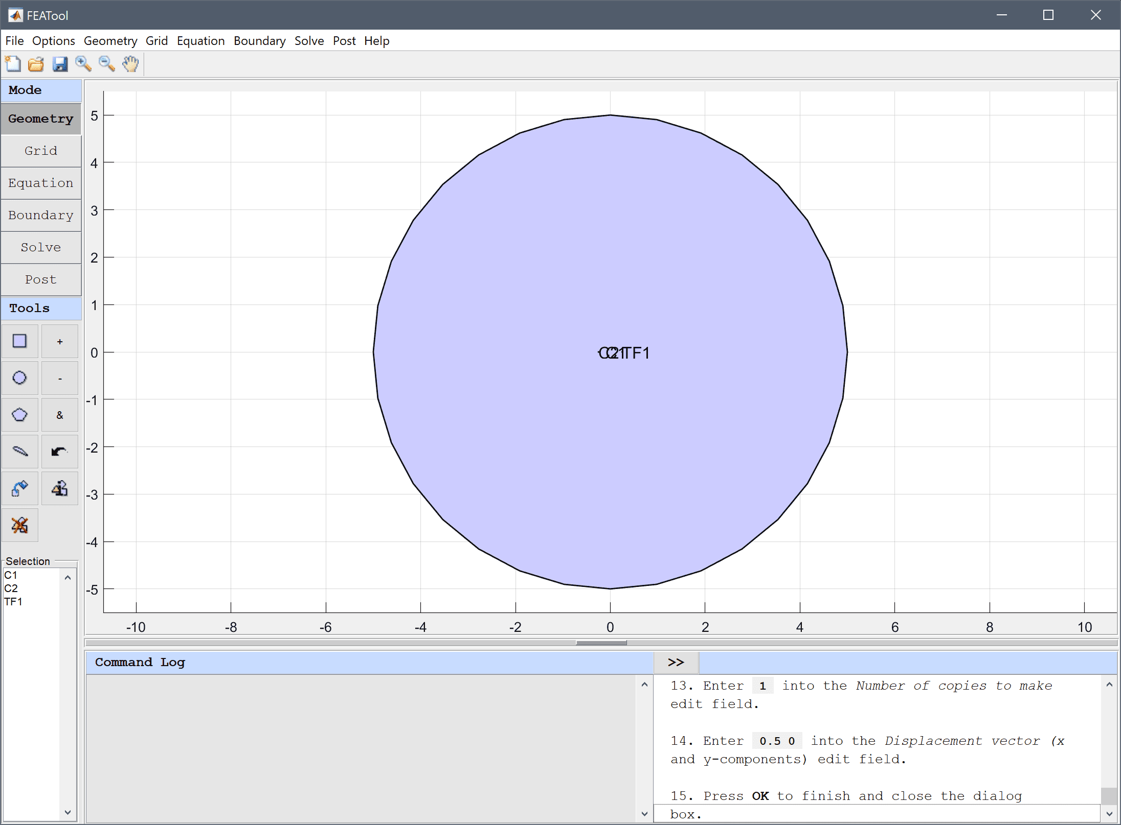
The basic domain is a circle centered at (0, 0) with radius 5 m.
5 into the radius edit field.Now create two circles 0.5 m apart each with radius 4 mm for the wire cross sections.
-0.25 0 into the center edit field.4e-3 into the radius edit field.The second wire can be created by copying and offsetting the first.
1 into the Number of copies to make edit field.0.5 0 into the Displacement vector (x and y-components) edit field.Press OK to finish and close the dialog box.
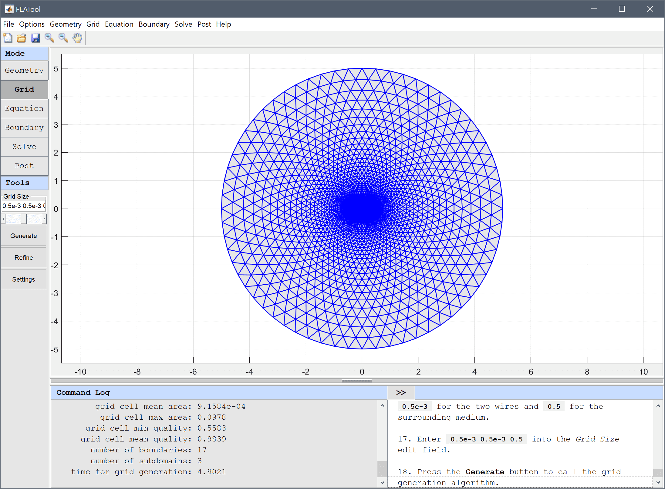
One can specify mesh sizes per subdomain by entering a space separated list of target mesh sizes in the Grid Size edit field (switch to Subdomain/Equation mode to see the domain order and numbering). Here we use target grid sizes of 0.5e-3 for the two wires and 0.5 for the surrounding medium.
0.5 0.5e-3 0.5e-3 into the Grid Size edit field.Press the Generate button to call the grid generation algorithm.
4*pi*1e-7 H/m, and the wires with opposite current densities of 1/(pi*0.004^2) A/m2. Note that FEATool does not enforce any specific unit system, but it is up to the user to select and use consistent units.4*pi*1e-7 into the Permeability edit field.Enter 0 into the Current density, z edit field.
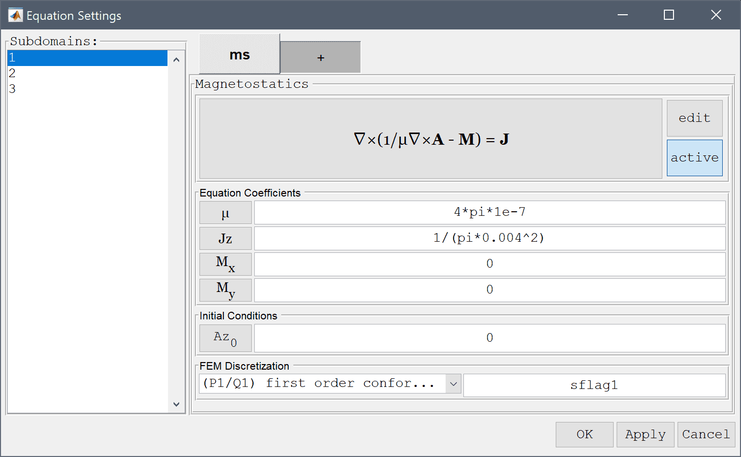
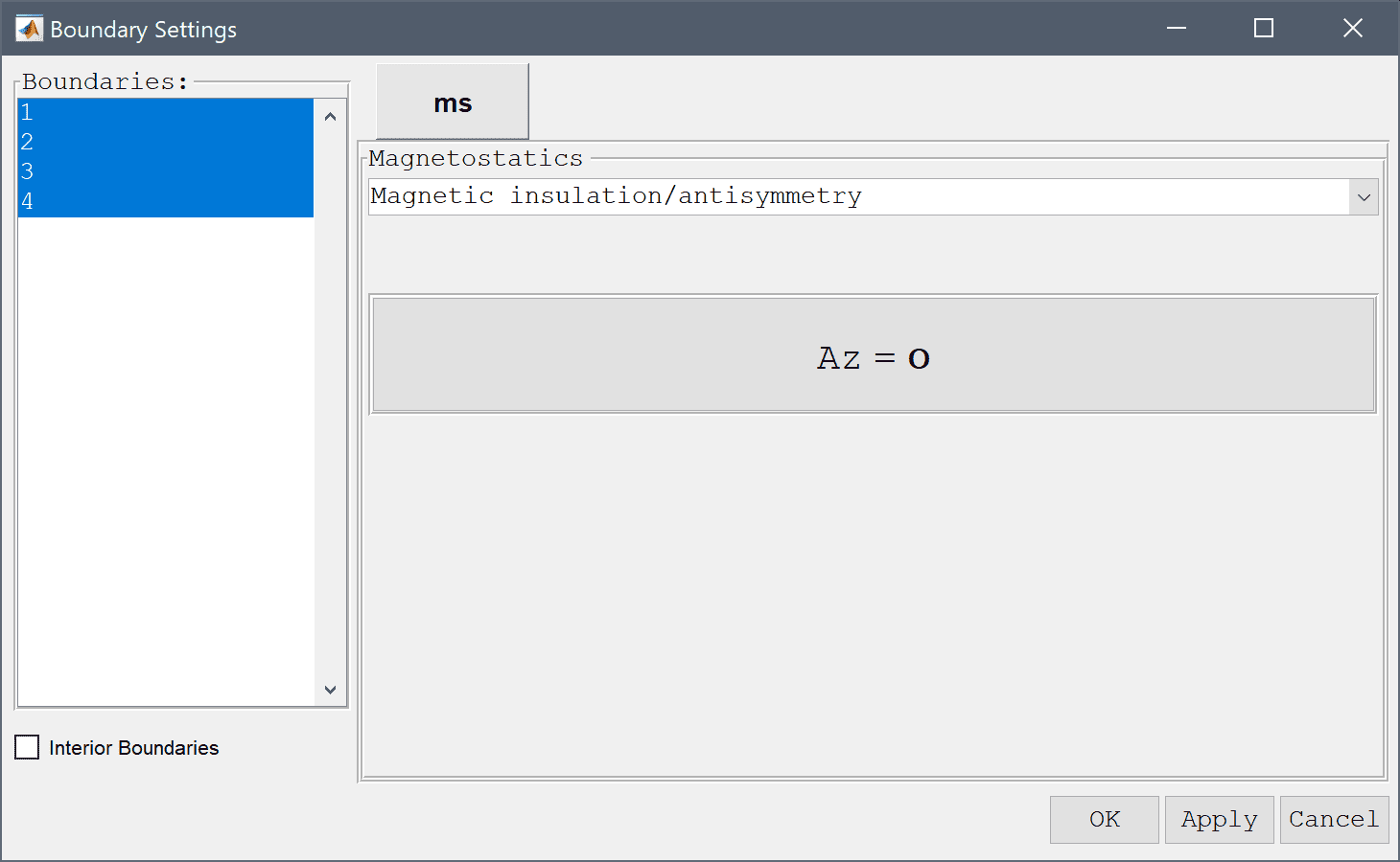
4*pi*1e-7 into the Permeability edit field.1/(pi*0.004^2) into the Current density, z edit field.4*pi*1e-7 into the Permeability edit field.-1/(pi*0.004^2) into the Current density, z edit field.Select the Magnetic insulation, Az = 0 boundary condition for all the outer boundaries.
Select Magnetic insulation/antisymmetry from the Magnetostatics drop-down menu.
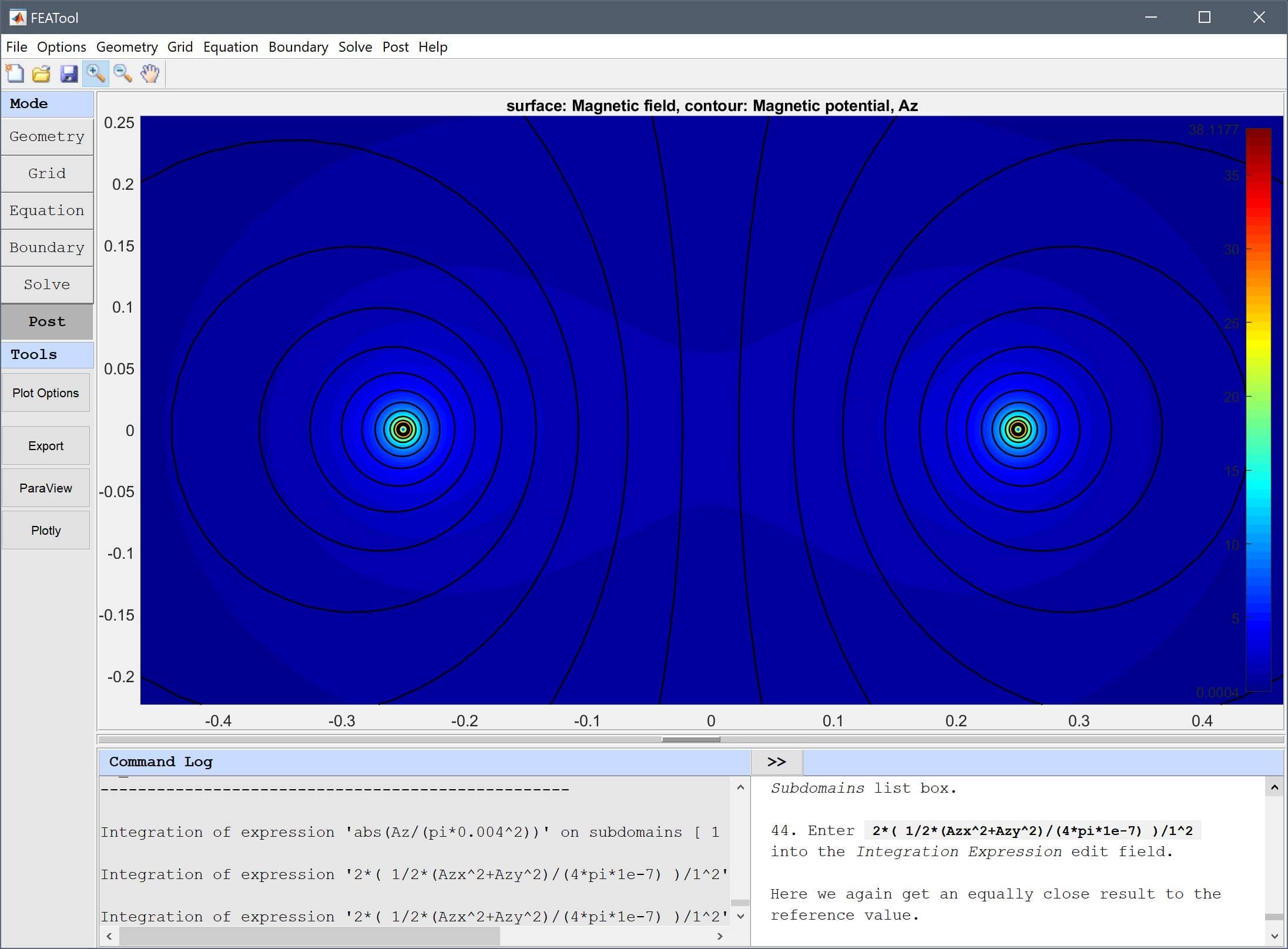
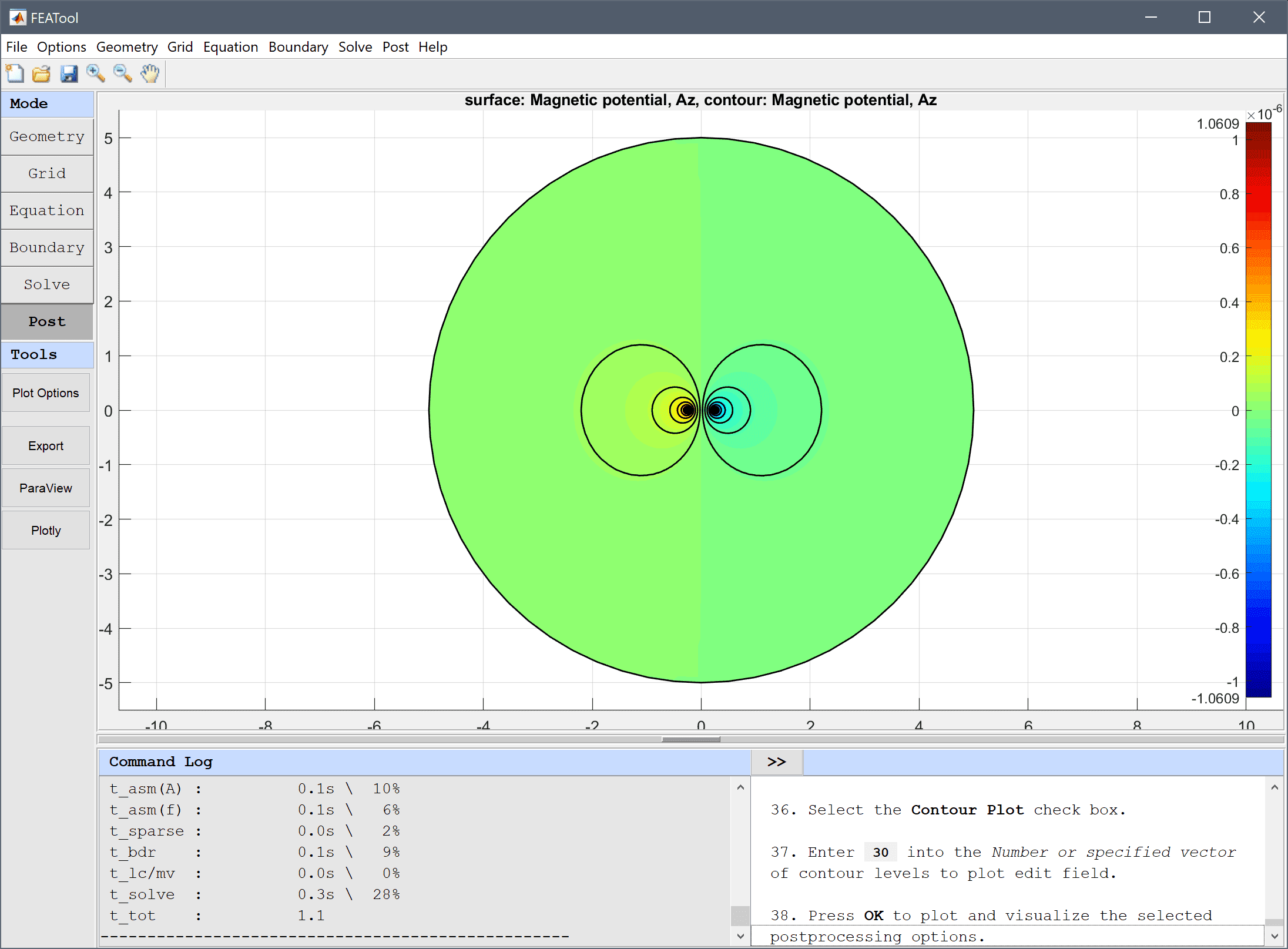
Select and plot the Magnetic potential, Az with contour lines and use the zoom button in the upper toolbar to zoom in on the wires.
30 into the Number or specified vector of contour levels to plot edit field.Press OK to plot and visualize the selected postprocessing options.
To compare the accuracy of the solution we first calculate the flux linkage by integrating the magnetic potential abs(Az/(pi*0.004^2)) per area over the wires, and dividing by the current 1 A.
abs(Az/(pi*0.004^2)) into the Integration Expression edit field.Press the Apply button.
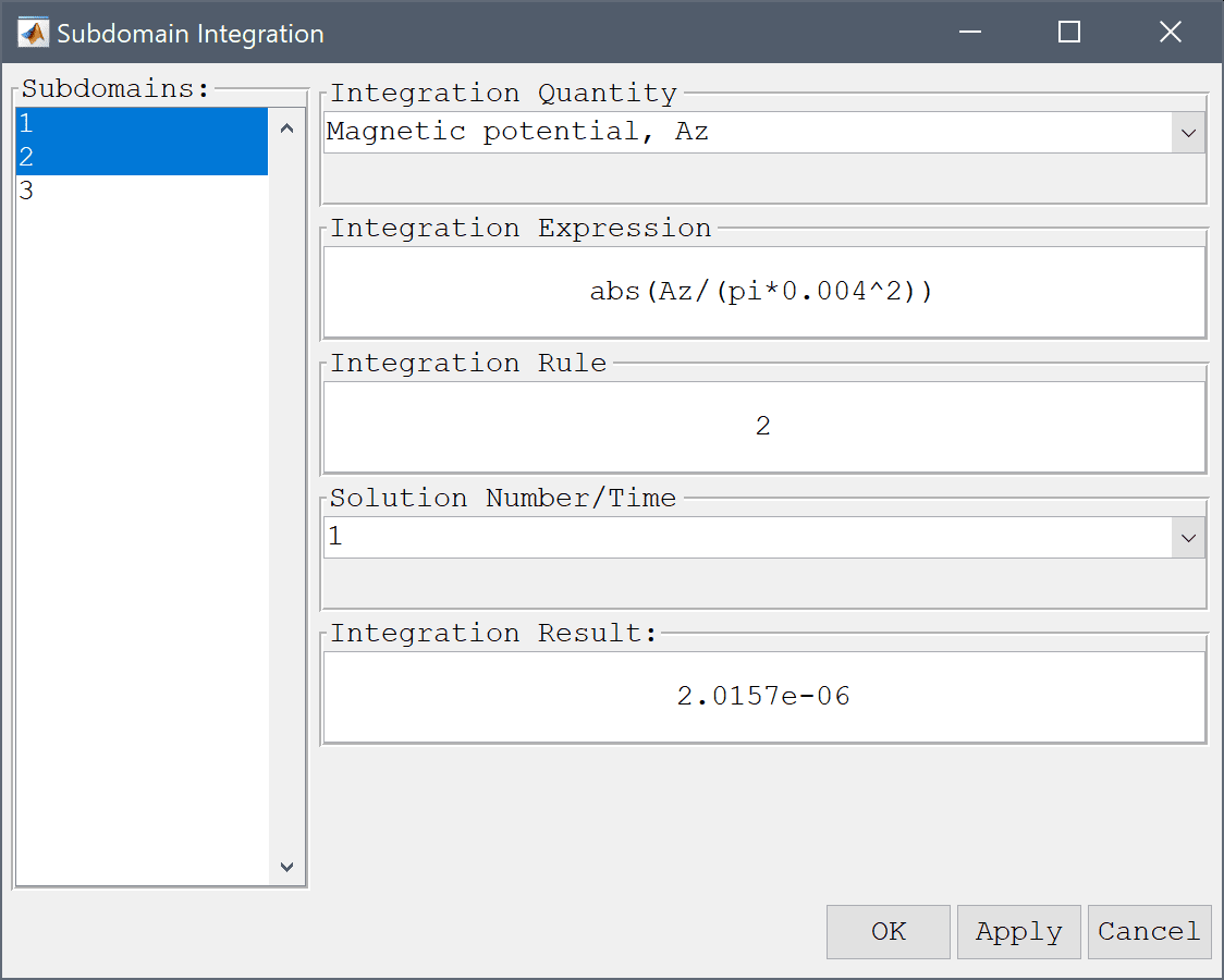
This results in a inductance value of 2.0157e-6 H which compares very well with the theoretical value of 2.0313e-06 H.
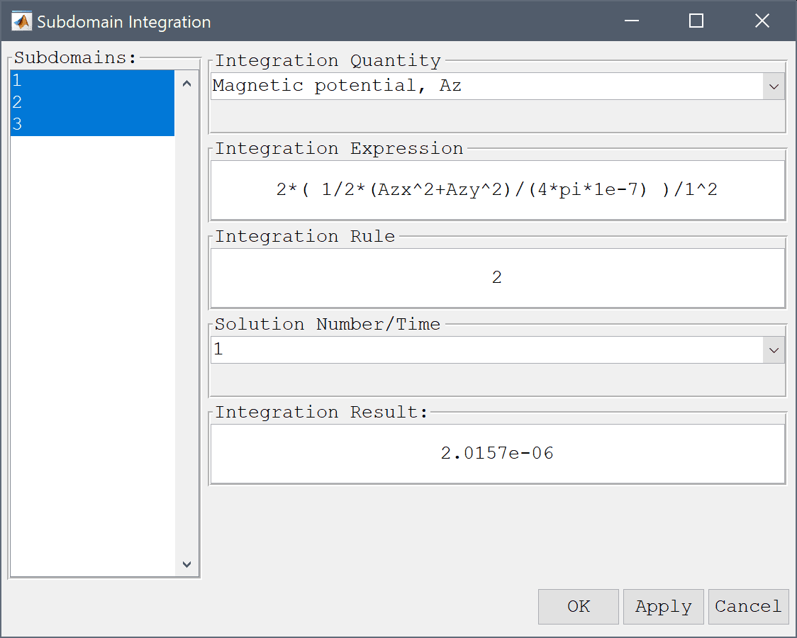
Another way to compute the inductance is to first calculate the total magnetic field energy W = 1/2∫(B⋅E)dV so that the inductance is given by L = 2W/I2. This is done in the following steps.
2*( 1/2*(Azx^2+Azy^2)/(4*pi*1e-7) )/1^2 into the Integration Expression edit field.Here we again get an equally close result to the reference value.
Press the Apply button.
The inductance in parallel wires electromagnetics model has now been completed and can be saved as a binary (.fea) model file, or exported as a programmable MATLAB m-script text file, or GUI script (.fes) file.