Capacitance in a Microstrip Transmission Line

A shielded electrical microstrip transmission line is fixed to a substrate and placed in a shielded container of air. The simulation applies a known voltage to the strip to calculate the resulting capacitance and compares this with the theoretical result. The problem assumes symmetry in the lengthwise direction so that the model can be reduced to a 2D planar cross-section. The strip is represented by an internal boundary to which the voltage is applied.

This model is available as an automated tutorial by selecting Model Examples and Tutorials... > Electromagnetics > Microstrip Transmission Line from the File menu. Or alternatively, follow the step-by-step instructions below.

Tutorial

1. To start a new model click the New Model toolbar button, or select New Model... from the File menu.

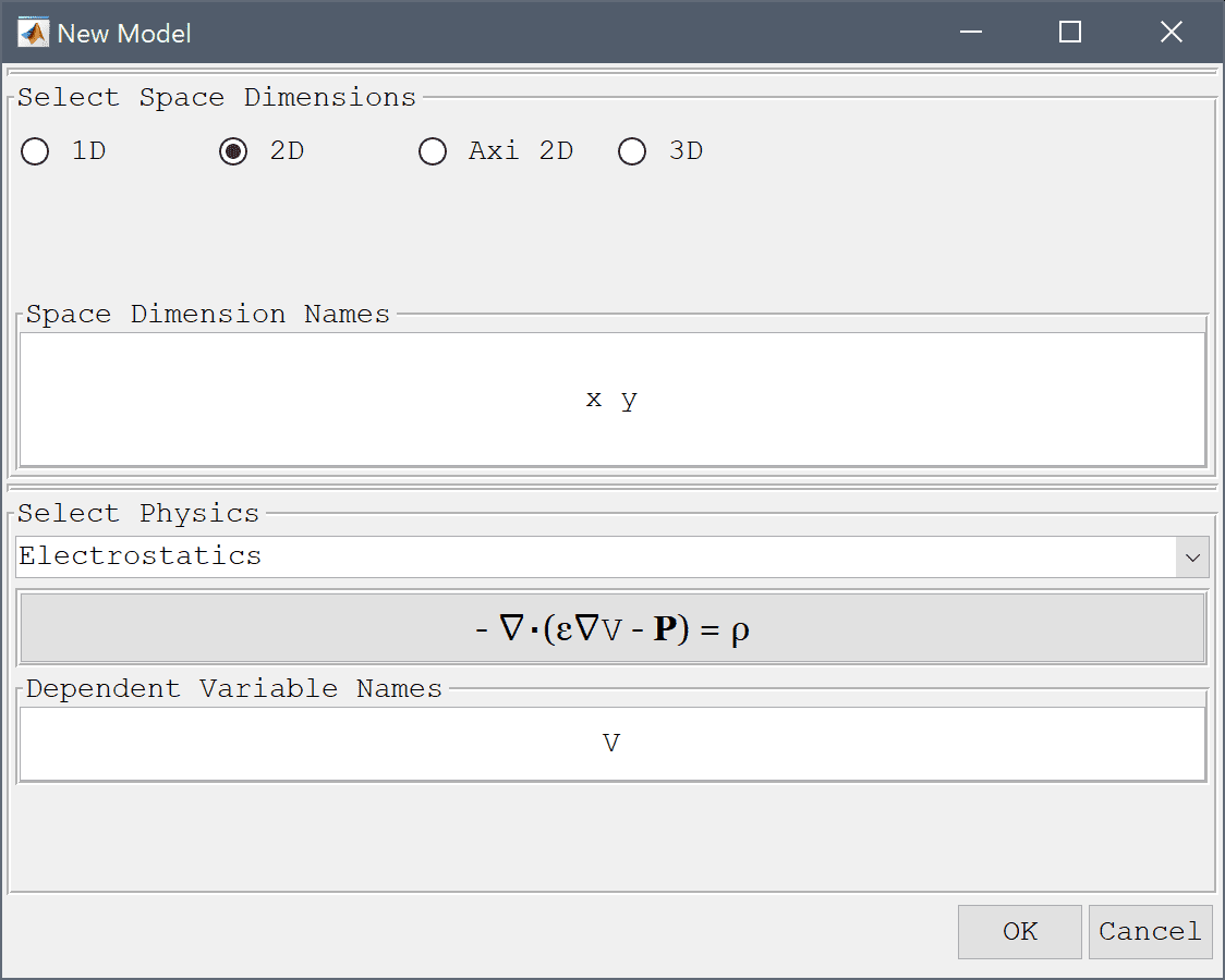
2. Select the Electrostatics physics mode from the Select Physics drop-down menu.

   
3. Press OK to finish the physics mode selection.

The geometry consists of a 0.1 x 0.09 m rectangle, representing the air, above a 0.1 x 0.01 m rectangle for the substrate.

1. Select Rectangle from the Geometry menu.
2. In the Edit Geometry Object dialog box, change the x/y_min and x/y_max point coordinates to define a rectangle with length 0.1 and height 0.09 and lower left corner at the origin (0, 0). Finish editing the geometry object and close the dialog box by clicking OK.
3. Enter 0 into the x_min edit field.
4. Enter 0.1 into the x_max edit field.
5. Enter 0.01 into the y_min edit field.

6. Enter 0.1 into the y_max edit field.

   
7. Press OK to finish and close the dialog box.
8. Select Rectangle from the Geometry menu.
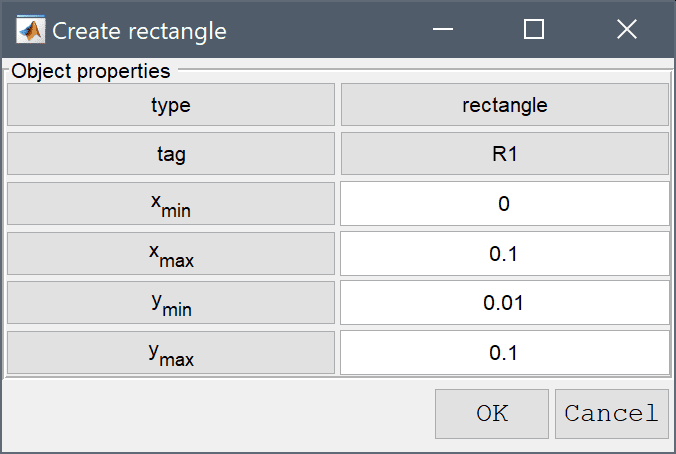
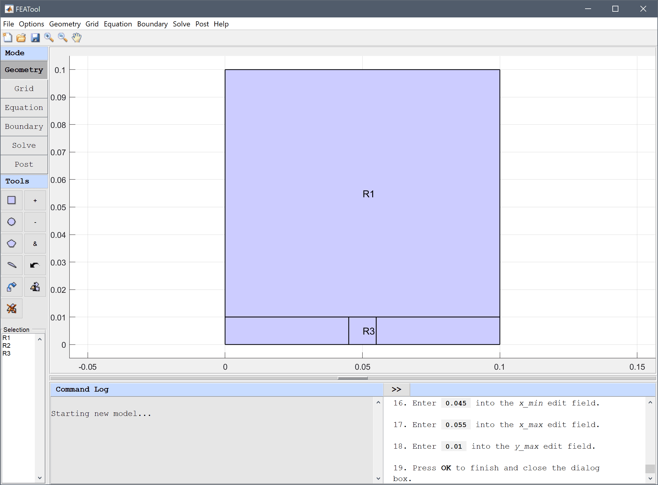
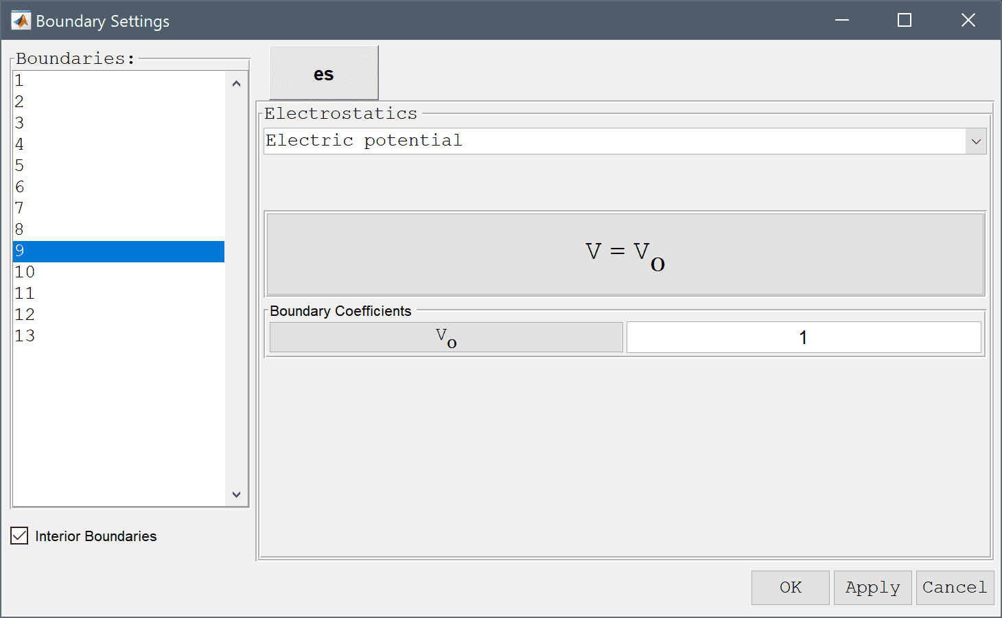
9. Enter 0.1 into the x_max edit field.
10. Enter 0.01 into the y_max edit field.
11. Press OK to finish and close the dialog box.

To represent the microstrip a 0.01 m interior border is required, to ensure this a third rectangle is created to split the substrate along the microstrip.

1. Select Rectangle from the Geometry menu.
2. Enter 0.045 into the x_min edit field.
3. Enter 0.055 into the x_max edit field.
4. Enter 0.01 into the y_max edit field.

5. Press OK to finish and close the dialog box.

   
6. Switch to Grid mode by clicking on the corresponding Mode Toolbar button.

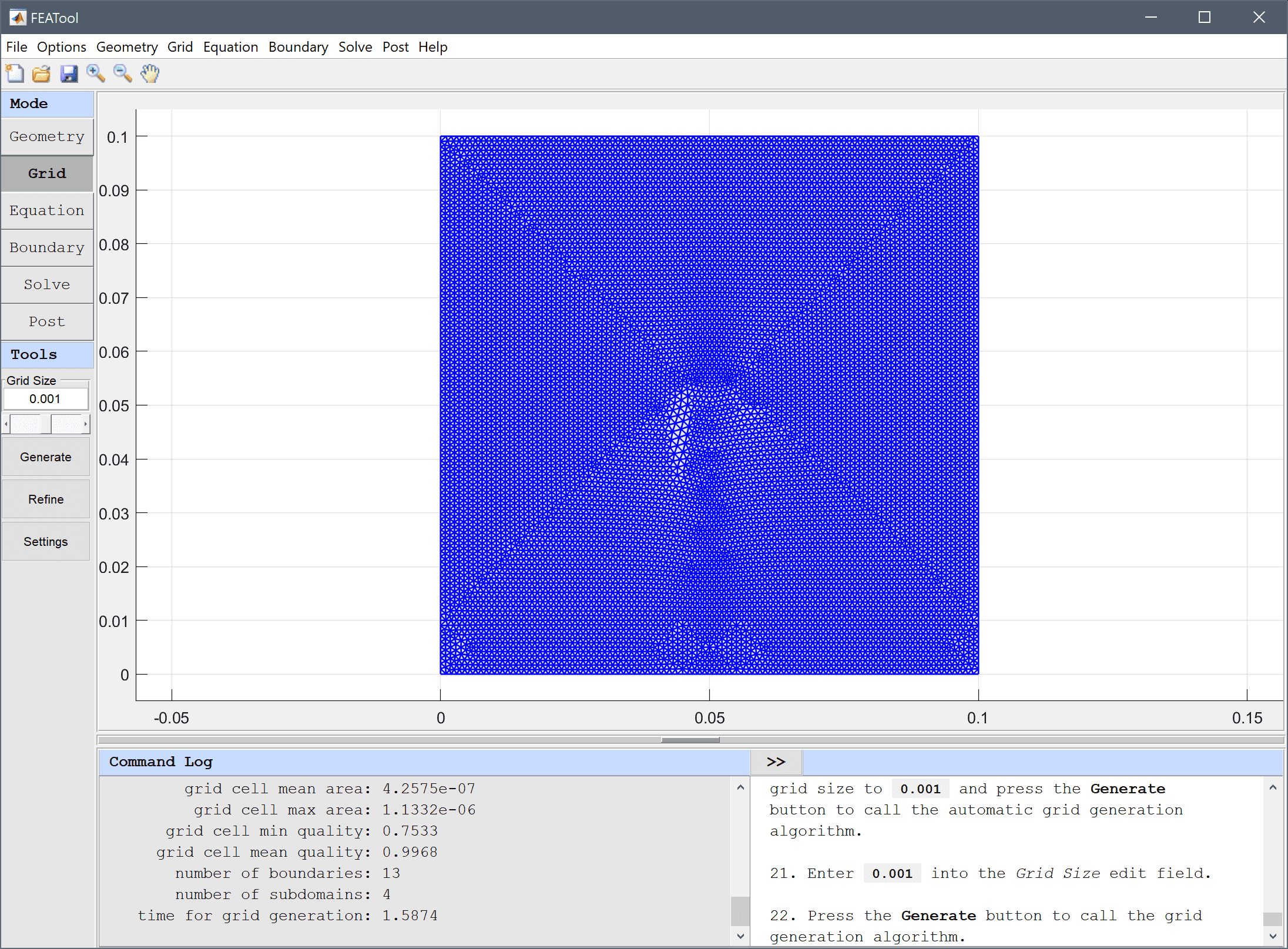
The default grid may be too coarse to ensure an accurate solution. Decrease the target subdomain grid size to 0.001 and press the Generate button to call the automatic grid generation algorithm.

1. Enter 0.001 into the Grid Size edit field.

2. Press the Generate button to call the grid generation algorithm.

   
3. Switch to Equation mode by clicking on the corresponding Mode Toolbar button.

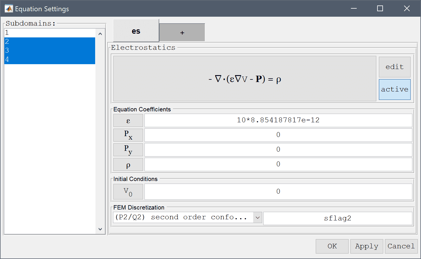
Equation and material coefficients can be specified in Equation/Subdomain mode. In the Equation Settings dialog box that automatically opens, enter the permittivities ε_rε₀, with the relative permittivity ε_r equal to 1 and 10 in the air and substrate, respectively. The other coefficients can be left to their default values.

1. Select 1 in the Subdomains list box.
2. Enter 1*8.854187817e-12 into the Permittivity edit field.
3. Select 2, 3, and 4 in the Subdomains list box.
4. Enter 10*8.854187817e-12 into the Permittivity edit field.

As the final quantities to compute involve derivatives of the potential a higher order solution space will enable higher accuracy.

1. Select (P2/Q2) second order conforming from the FEM Discretization drop-down menu.

   
2. Press OK to finish the equation and subdomain settings specification.

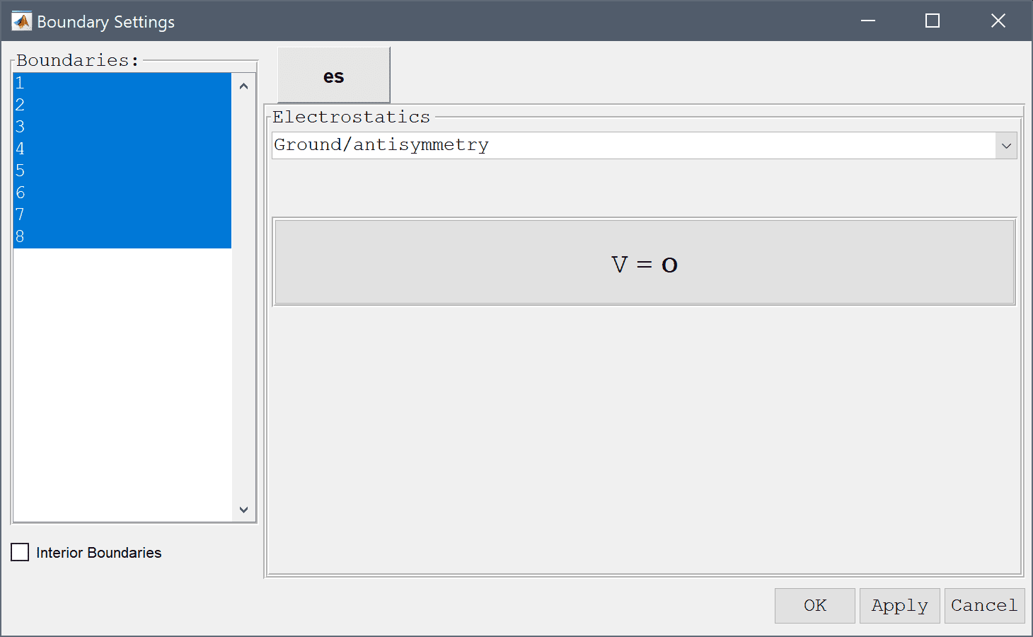
Boundary conditions are defined in Boundary Mode and describes how the model interacts with the external environment. The external boundaries (1-8) represent the shield and should be connected to the ground with zero potential.

1. Switch to Boundary mode by clicking on the corresponding Mode Toolbar button.
2. Select the external boundaries (1-8) in the Boundaries list box.

3. Select Ground/antisymmetry from the Electrostatics drop-down menu.

   
4. The microstrip should be set to a potential of 1 V. Mark the Interior Boundaries checkbox to enable selection of boundary conditions for internal boundaries.
5. Select 10 in the Boundaries list box.
6. Select Electric potential from the Electrostatics drop-down menu.

7. Enter 1 into the Surface charge edit field.

   
8. Press OK to finish the boundary condition specification.
9. Now that the problem is fully specified, press the Solve Mode Toolbar button to switch to solve mode. Then press the = Tool button to call the solver with the default solver settings.
10. To add contour lines to the plot, first open the postprocessing settings dialog box by clicking on the Plot Options Toolbar button.
11. Select the Contour Plot check box.

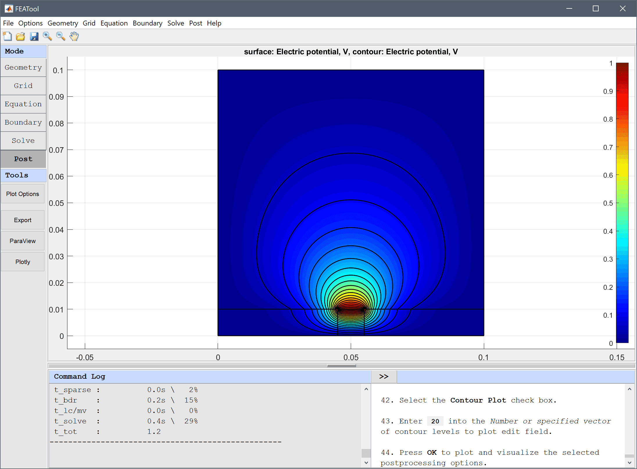
12. Enter 20 into the Number or specified vector of contour levels to plot edit field.

    

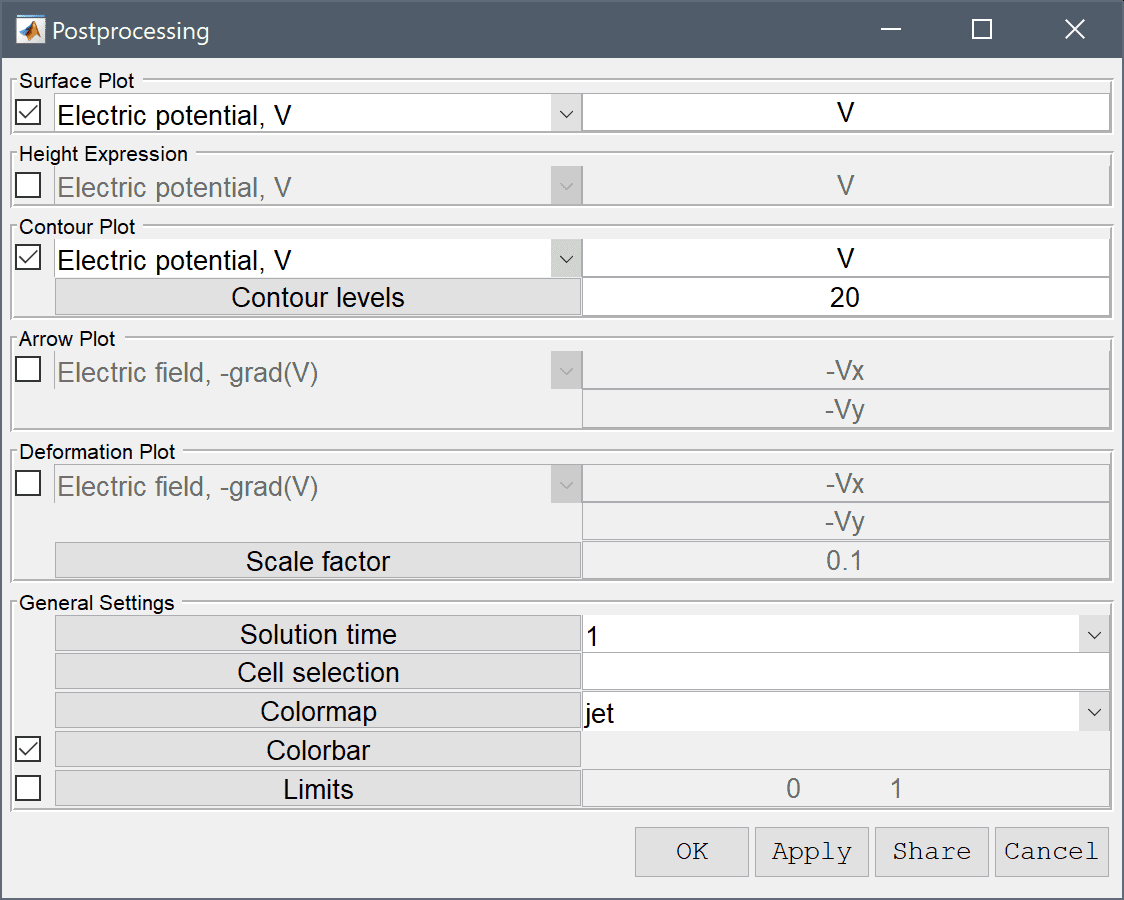
13. Press OK to plot and visualize the selected postprocessing options.

    

To validate the solution we will compute the capacitance with two approaches and compare with the theoretical result of C = 178.1 pF.

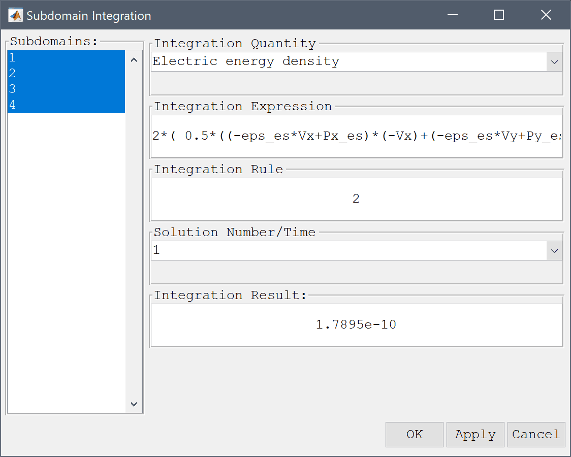
The first approach is to calculate the total stored energy of the electric field W, and as the voltage U is known, then the capacitance follows as C = 2W/U².

1. Select Subdomain Integration... from the Post menu.
2. Select Electric energy density from the Predefined integration expressions drop-down menu.

Modify the expression to account for the energy factor 2 and division by the voltage squared.

1. Enter 2*( 0.5*((-eps_es*Vx+Px_es)*(-Vx)+(-eps_es*Vy+Py_es)*(-Vy)) )/1^2 into the Integration Expression edit field.

2. Press the Apply button.

   

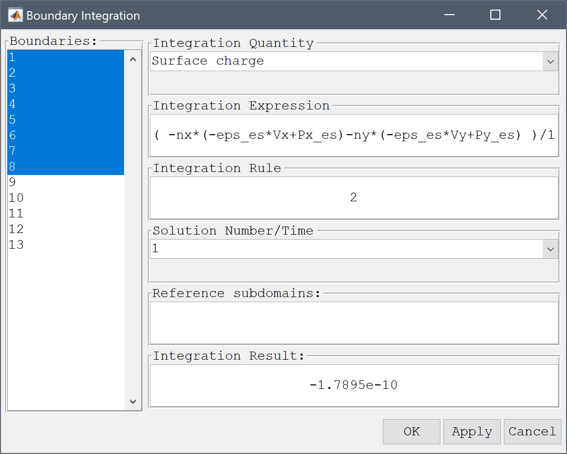
The second approach is to calculate the electric charge around the strip q and divide by the known voltage U.

1. Press OK to finish and close the dialog box.
2. Select Boundary Integration... from the Post menu.
3. Select 1-8 in the Boundaries list box.
4. Select Surface charge from the Predefined integration expressions drop-down menu.

Modify the expression to account for division by the voltage.

1. Enter ( -nx*(-eps_es*Vx+Px_es)-ny*(-eps_es*Vy+Py_es) )/1 into the Integration Expression edit field.

2. Press the Apply button.

   
3. Press OK to finish and close the dialog box.

Both approaches should yield results within 0.1 % of the theoretical expected result.

The microstrip transmission line electromagnetics model has now been completed and can be saved as a binary (.fea) model file, or exported as a programmable MATLAB m-script text file, or GUI script (.fes) file.