Skin effect is a phenomenon where an alternating current tends to flow and distribute itself along the surface layer or outside skin of a conductor. This effect can for example be taken advantage of in power transmission applications by layering inexpensive conductor materials (for example aluminium) with a thin layer of more conductive material (like copper). This model examines the skin effect in a two-dimensional cross section of a thick circular wire with an outer radius R = 12 cm.

A time-harmonic complex Helmholtz equation for the amplitude of the electric field E is used to model the skin effect

\[ -\nabla\cdot(\frac{1}{\mu}\nabla E) + k^2 E = 0 \]

where μ is the permeability 4π·10^-7 H/m, and the wave number k is given by

\[ k = \sqrt{i\omega\sigma - \omega^2\epsilon} \]

where σ is the conductivity of the material, ε the dielectic properties, and ω angular frequncy (here 60 Hz). Complex (and imaginary) numbers are denoted using the i coefficient.

The computed current density in a circular wire of homogenous material can be compared with the exact solution [1] as

\[ J(r) = \frac{k I}{2\pi R}\frac{J_0(k r)}{J_1(k R)} \]

where J_n is the Bessel function of the n:th order.

This model is available as an automated tutorial by selecting Model Examples and Tutorials... > Electromagnetics > Surface Currents in a Circular Wire from the File menu. Or alternatively, follow the step-by-step instructions below.

Tutorial

To start a new model click the New Model toolbar button, or select New Model... from the File menu.

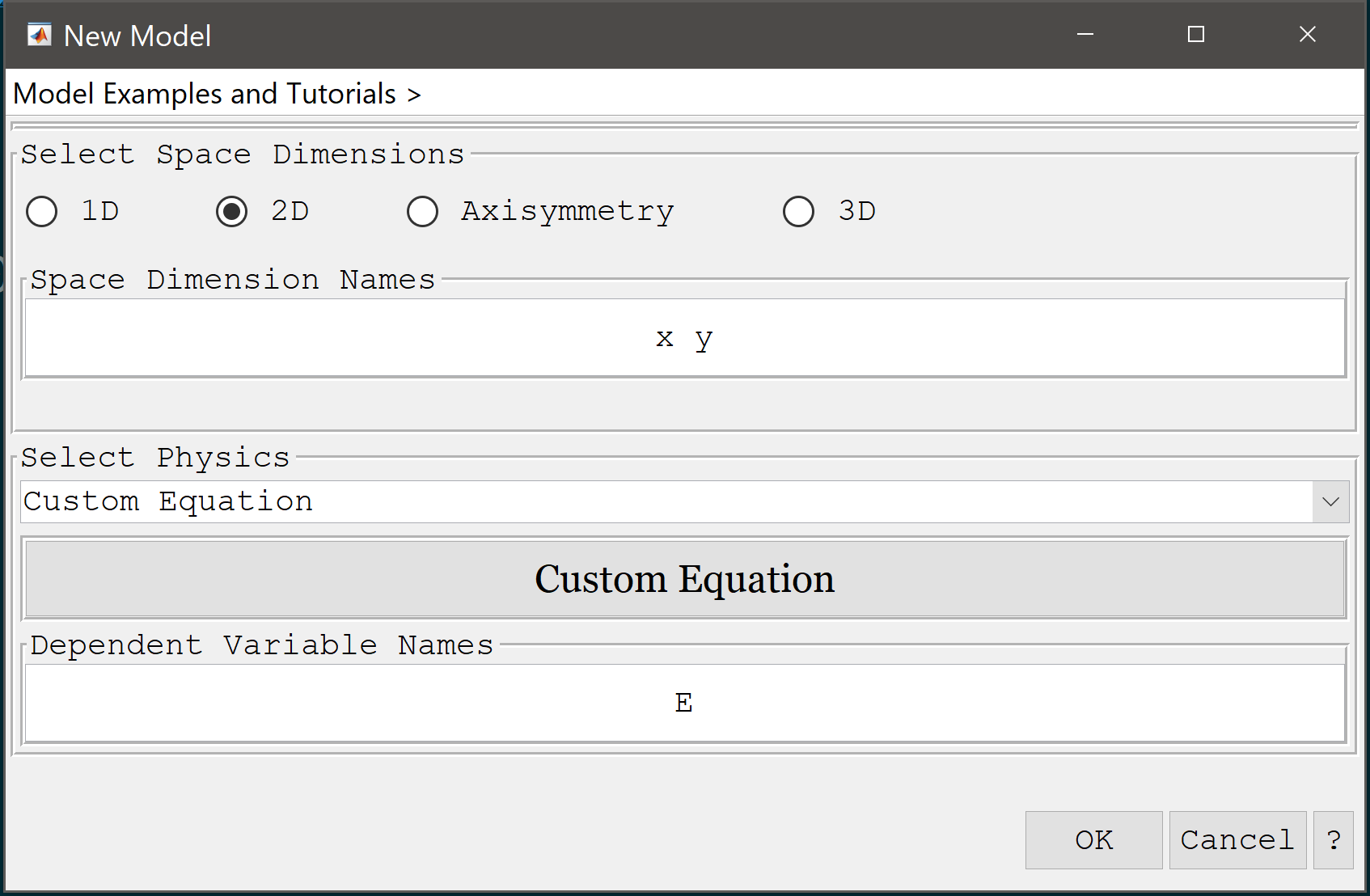
This tutorial will use the custom equation physics mode to define a time-harmonic Helmholtz PDE.

Select the Custom Equation physics mode from the Select Physics drop-down menu.

Change the dependent variable name to E, to represent the amplitude of the electric field.

Enter E into the Dependent Variable Names edit field.
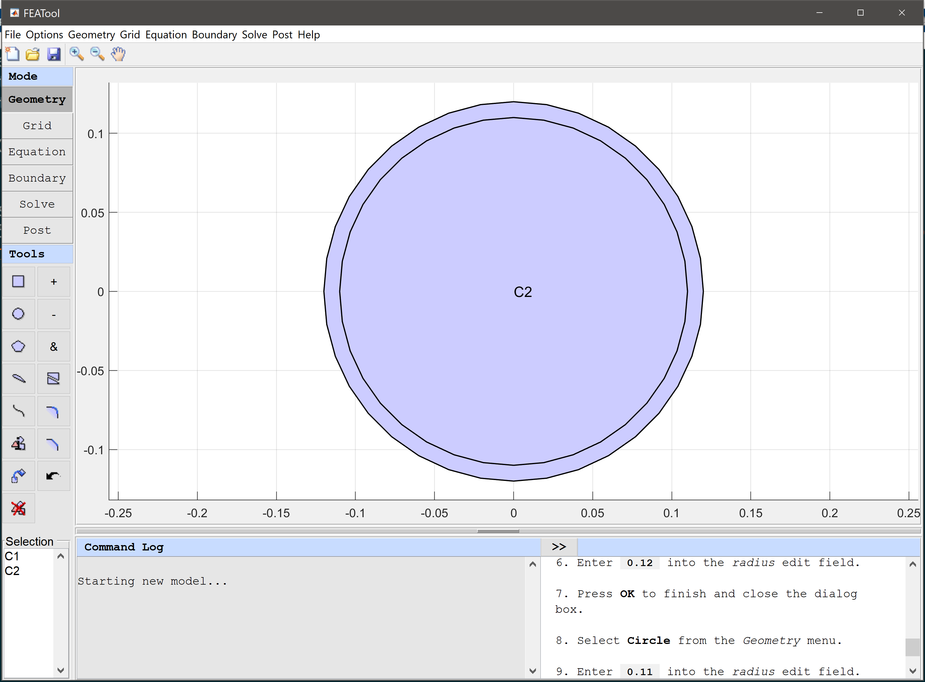
Press OK to finish the physics mode selection.

For the geometry, create two overlapping circles with radius 0.12 and 0.11 m, respectively.

Select Circle from the Geometry menu.
Enter 0.12 into the radius edit field.
Press OK to finish and close the dialog box.
Select Circle from the Geometry menu.
Enter 0.11 into the radius edit field.
Press OK to finish and close the dialog box.
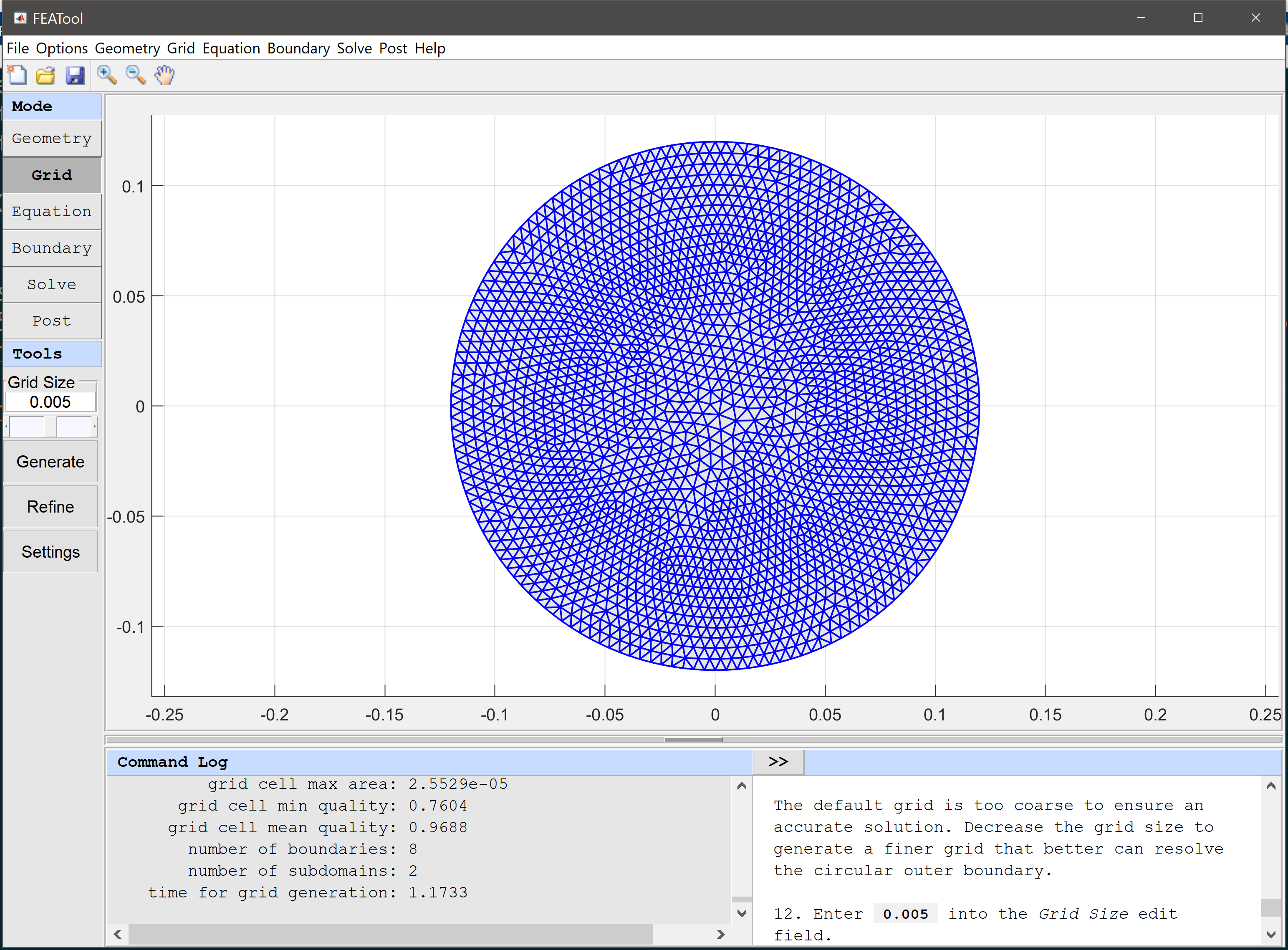
Switch to Grid mode by clicking on the corresponding Mode Toolbar button.

The default grid is too coarse to ensure an accurate solution. Decrease the grid size to generate a finer grid that better can resolve the circular outer boundary.

Enter 0.005 into the Grid Size edit field.
Press the Generate button to call the grid generation algorithm.
Switch to Equation mode by clicking on the corresponding Mode Toolbar button.
Select 1 and 2 in the Subdomains list box.
Press the edit button.

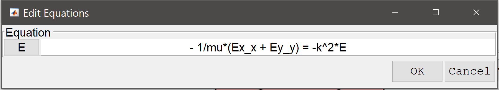
Change from the default Poisson equation to the Helmholtz equation in the Edit Equations dialog box.

Enter - 1/mu*(Ex_x + Ey_y) = -k^2*E into the Equation for E edit field.
Press OK to finish the equation and subdomain settings specification.
Press the Constants Toolbar button, or select the corresponding entry from the Equation menu, and add the following modeling constants for the speed of light, frequency, and wave number in the Model Constants and Expressions dialog box. (Note that entering a space separated list allows prescribing constants and expressions per subdomain.)

Name	Expression
mu	pi*4e-7
sigma_cu	6e7
sigma_al	3.8e7
sigma	sigma_cu
omega	2pi60
epsilon	8.854e-12
I	120
k	sqrt(iomegasigma-omega^2*epsilon)

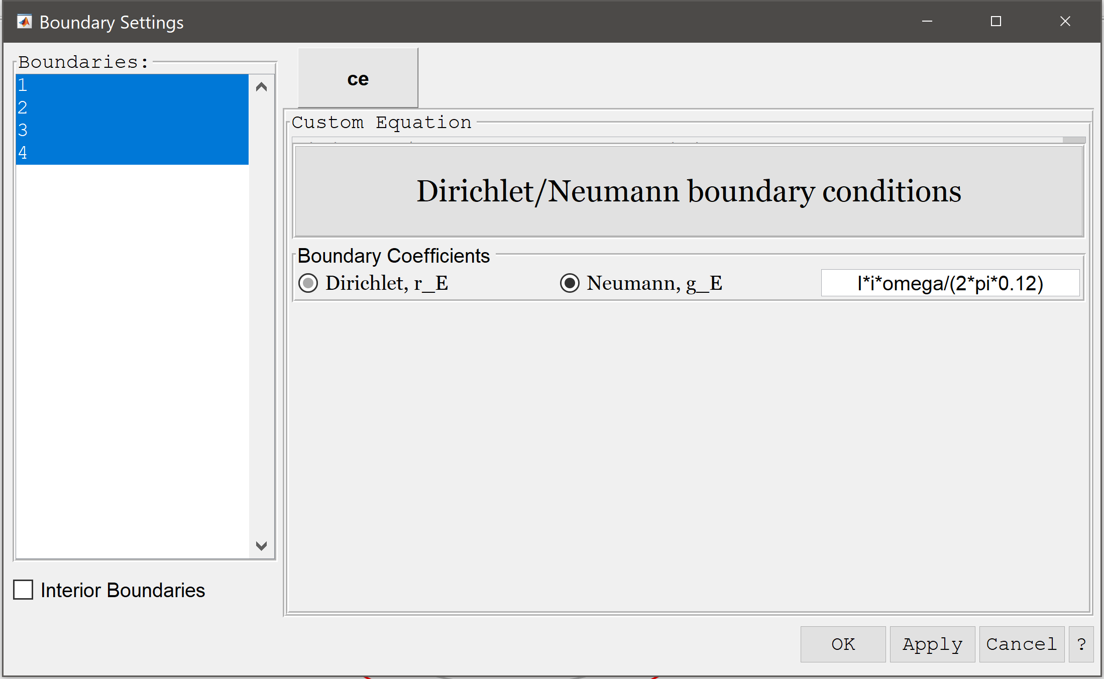
Switch to Boundary mode by clicking on the corresponding Mode Toolbar button.

In boundary mode, select Neumann conditions for all boundaries. The Neumann boundary coefficient should be prescribed so that the magnetic field vanishes outside the wire, here by specifying the equivalent negative surface current.

Select 1-4 in the Boundaries list box.
Select the Neumann, g_E radio button.
Enter I*i*omega/(2*pi*0.12) into the Dirichlet/Neumann coefficient edit field.
Press OK to finish the boundary condition specification.
Switch to Solve mode by clicking on the corresponding Mode Toolbar button.

It is required to use the backslash linear solver for complex valued solutions. Make sure it is selected in the Solver Settings dialog box.

Press the Settings Toolbar button.
Select backslash from the Linear solver selection drop-down menu.
Press OK to apply the selected solver settings.
Press the = Toolbar button to call the solver. After the problem has been solved FEATool will automatically switch to postprocessing mode and plot the computed solution.

After the problem has been solved FEATool will automatically switch to Postprocessing mode and show real part of the computed amplitude of the electric field.

As the solution is complex valued, we can plot the real, imaginary, and absolute magnitude of the solution using the real, imag, and abs functions.

Press the Plot Options Toolbar button.

Comparing the computed with analytical current density (using the Bessel function besseli) we can see that the computed errors are very small.

Enter real(sigma*E - I*sqrt(mu)*k/(2*pi*0.12)*besseli(0,sqrt(mu)*k*sqrt(x^2+y^2))/besseli(1,sqrt(mu)*k*0.12)) into the Surface plot expression edit field.
Press Apply to plot and visualize the error in computed surface current.
Enter sigma*E into the Surface plot expression edit field and press OK to plot and visualize the surface current.

By integrating the current density over the cross-section we can also see that it is very close to the prescribed 120 A/m².

Select Subdomain Integration... from the Post menu.
Enter sigma*E into the Integration Expression edit field.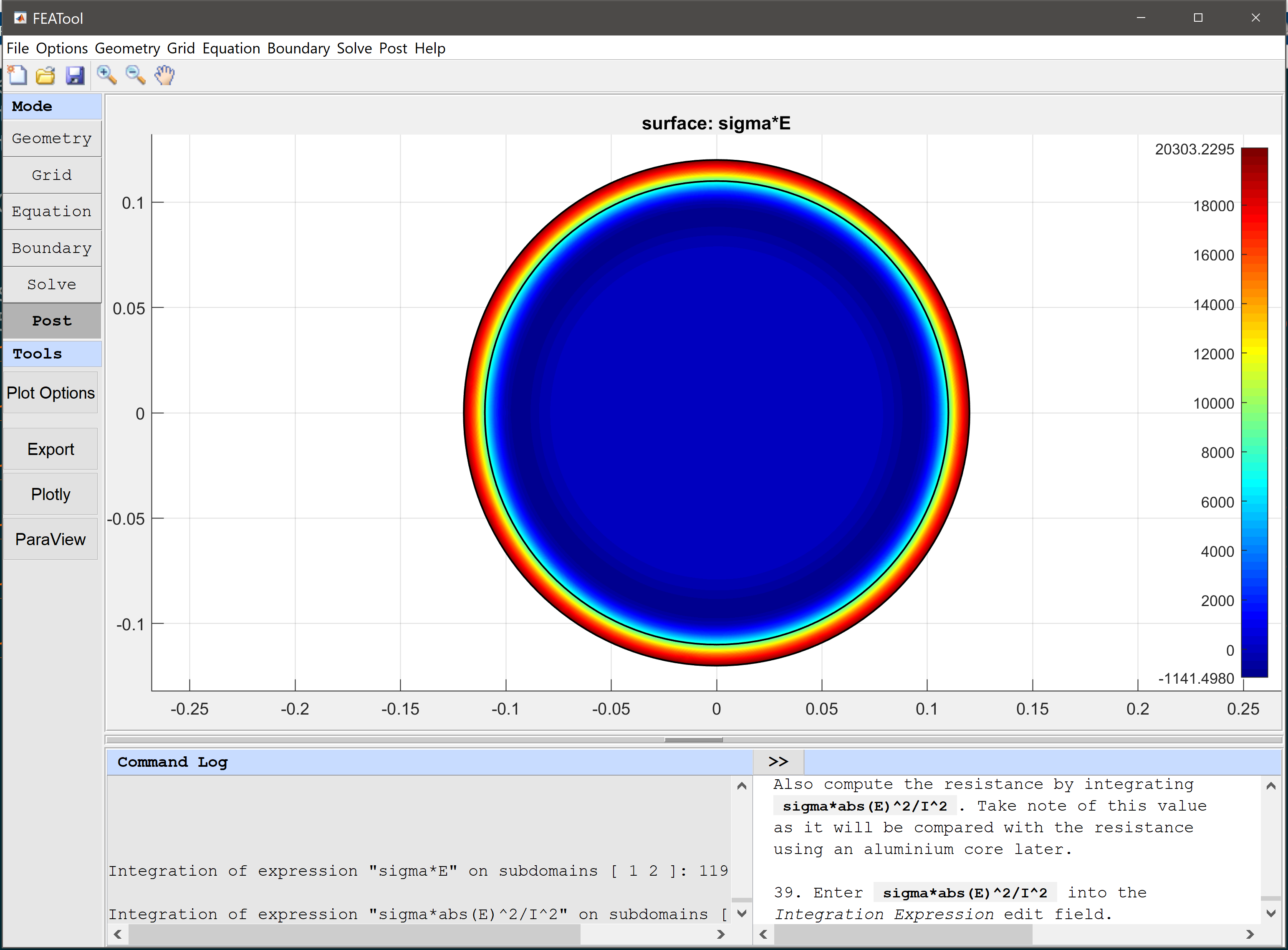
Press the Apply button.

Also compute the resistance by integrating sigma*abs(E)^2/I^2. Take note of this value as it will be compared with the resistance using an aluminium core later.

Enter sigma*abs(E)^2/I^2 into the Integration Expression edit field.
Press OK to finish and close the dialog box.

Now we want to change the material of the core subdomain to aluminium. To do this open the Model Constants dialog box again and change the conductivity to sigma_cu sigma_al. This will use conductivity of copper in the first (outer) subdomain, and that of aluminium in the second (inner).

Select Model Constants and Expressions... from the Equation menu.
Enter sigma_cu sigma_al into the expression edit field for the conductivity sigma.
Press OK to finish and close the dialog box.
Switch to Solve mode by clicking on the corresponding Mode Toolbar button.
Press the = Toolbar button to call the solver again.
Select Subdomain Integration... from the Post menu.
Enter sigma*abs(E)^2/I^2 into the Integration Expression edit field.
Press OK to finish and close the dialog box.

After calculating the new resistivity we can see that using a cheaper aluminium core does not significantly decrease the efficiency of the wire.

The surface currents in a circular wire electromagnetics model has now been completed and can be saved as a binary (.fea) model file, or exported as a programmable MATLAB m-script text file, or GUI script (.fes) file.

Reference

[1] Weeks, Walter L. (1981), Transmission and Distribution of Electrical Energy, Harper & Row, ISBN 978-0060469825.