Flow in Driven Cavity

Stationary and laminar incompressible flow in a square cavity (Reynolds number, Re = 1000). The top of the cavity is prescribed a tangential velocity while the sides and bottom are defined as no-slip zero velocity walls.

Tutorial

This model is available as an automated tutorial by selecting Model Examples and Tutorials... > Fluid Dynamics > Flow in Driven Cavity from the File menu. Or alternatively, follow the step-by-step instructions below. Note that the CFDTool interface differ slightly from the FEATool Multiphysics instructions described in the following.

1. To start a new model click the New Model toolbar button, or select New Model... from the File menu.
2. Select the 2D radio button.

3. Select the Navier-Stokes Equations physics mode from the Select Physics drop-down menu. (Note that for CFDTool the physics selection is done in the Equation settings dialog box.)

   
4. Press OK to finish the physics mode selection.

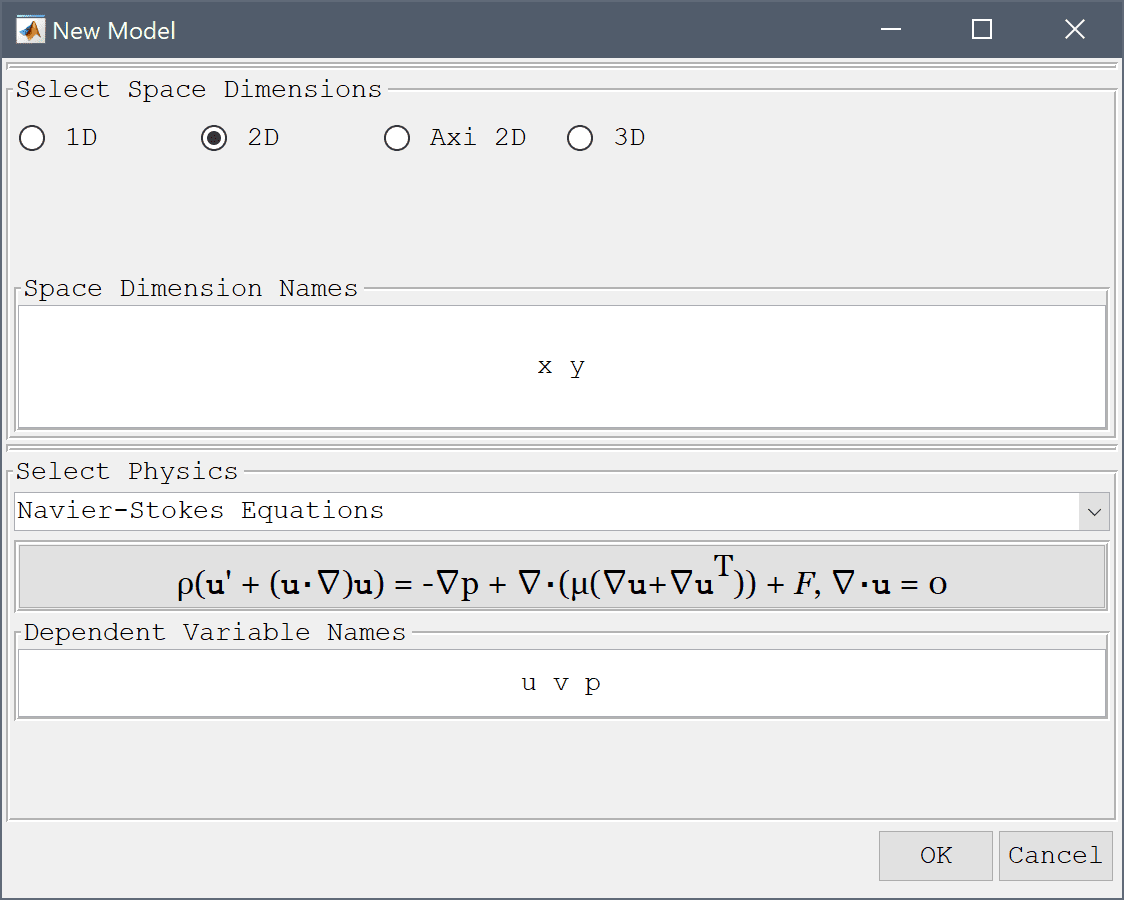
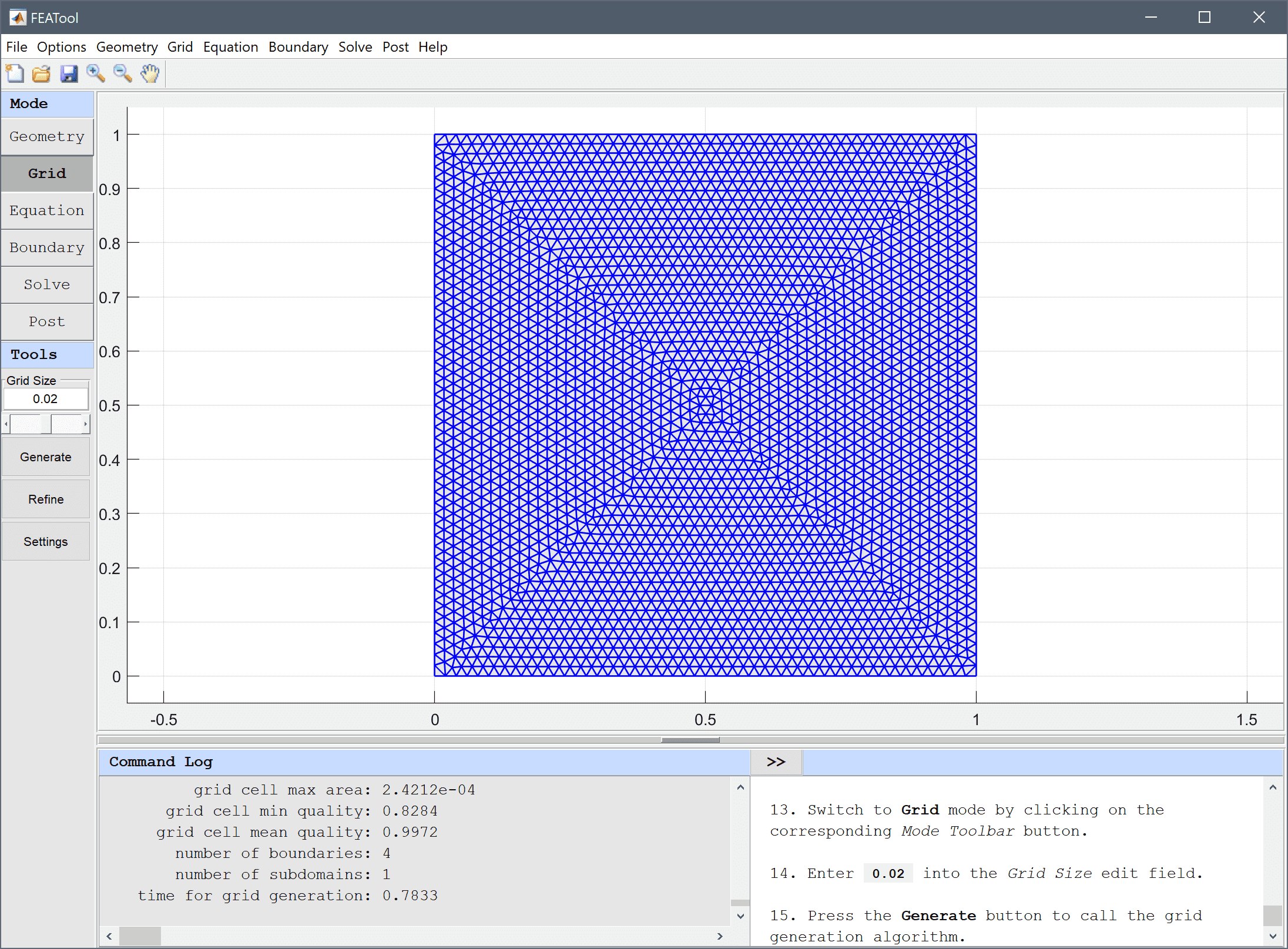
First create a unit square for the geometry.

1. To create a rectangle, first click on the Create square/rectangle Toolbar button. Then left click in the main plot axes window, and hold down the mouse button. Move the mouse pointer to draw the shape outline, and release the button to finalize the shape.
2. Select R1 in the geometry object Selection list box.
3. To modify and edit the selected rectangle, click on the Inspect/edit selected geometry object Toolbar button to open the Edit Geometry Object dialog box.
4. Enter 0 into the x_min edit field.
5. Enter 1 into the x_max edit field.
6. Enter 0 into the y_min edit field.
7. Enter 1 into the y_max edit field.
8. Press OK to finish and close the dialog box.
9. Switch to Grid mode by clicking on the corresponding Mode Toolbar button.
10. Enter 0.02 into the Grid Size edit field.

11. Press the Generate button to call the grid generation algorithm.

    
12. Switch to Equation mode by clicking on the corresponding Mode Toolbar button.

13. Equation and material coefficients can be specified in Equation/Subdomain mode. In the Equation Settings dialog box that automatically opens, enter 1 for the fluid Density and umax/l/R for the Viscosity. The other coefficients can be left to their default values. Press OK to finish the equation and subdomain settings specification. (Note that the Equation Settings dialog box may look different for CFDTool.)

    

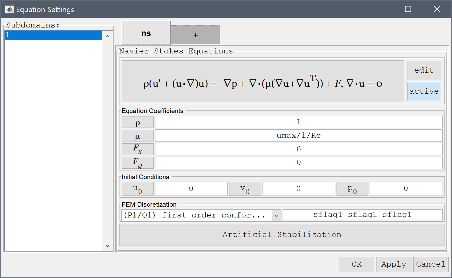
Note that FEATool works with any unit system, and that the units here are non-dimensionalized.

1. Press the Constants Toolbar button, or select the corresponding entry from the Equation menu, and enter the variables for the velocity umax, length l, and Reynolds number Re in the Model Constants and Expressions dialog box.

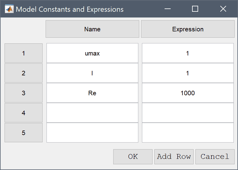
Name	Expression
umax	1
l	1
Re	1000

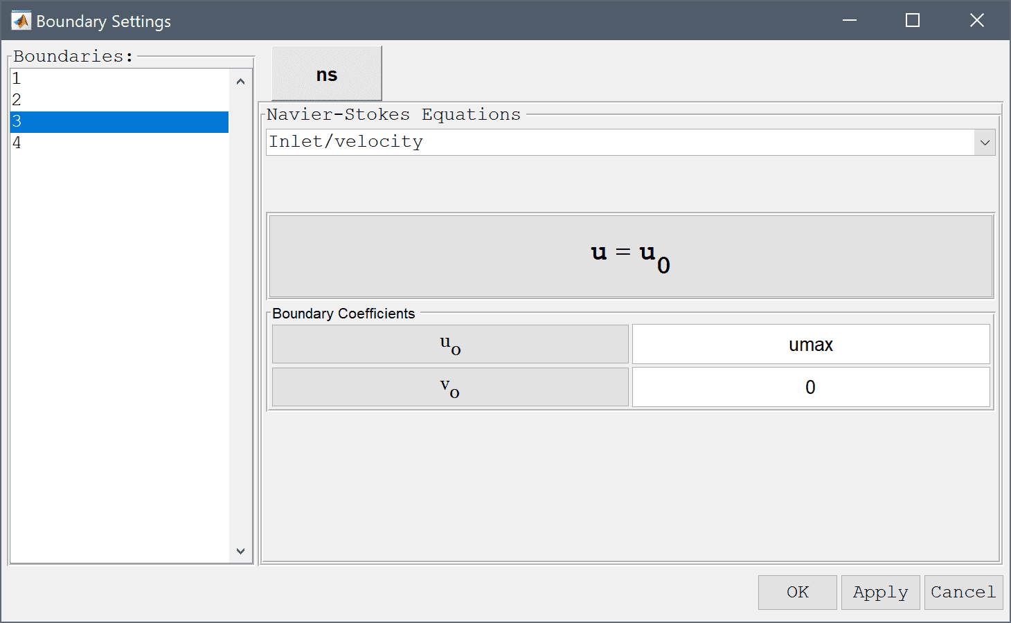
Boundary conditions consist of no-slip zero velocity conditions on all walls except for the top on which a constant x-velocity umax is prescribed.

1. Switch to Boundary mode by clicking on the corresponding Mode Toolbar button.
2. Select 4 in the Boundaries list box.
3. Select 1, 2, 3, and 4 in the Boundaries list box.
4. Select Wall/no-slip from the Navier-Stokes Equations drop-down menu.
5. Select 3 in the Boundaries list box.
6. Select Inlet/velocity from the Navier-Stokes Equations drop-down menu.

7. Enter umax into the Velocity in x-direction edit field.

   
8. Press OK to finish the boundary condition specification.

9. Now that the problem is fully specified, press the Solve Mode Toolbar button to switch to solve mode. Then press the = Tool button to call the solver with the default solver settings.

   

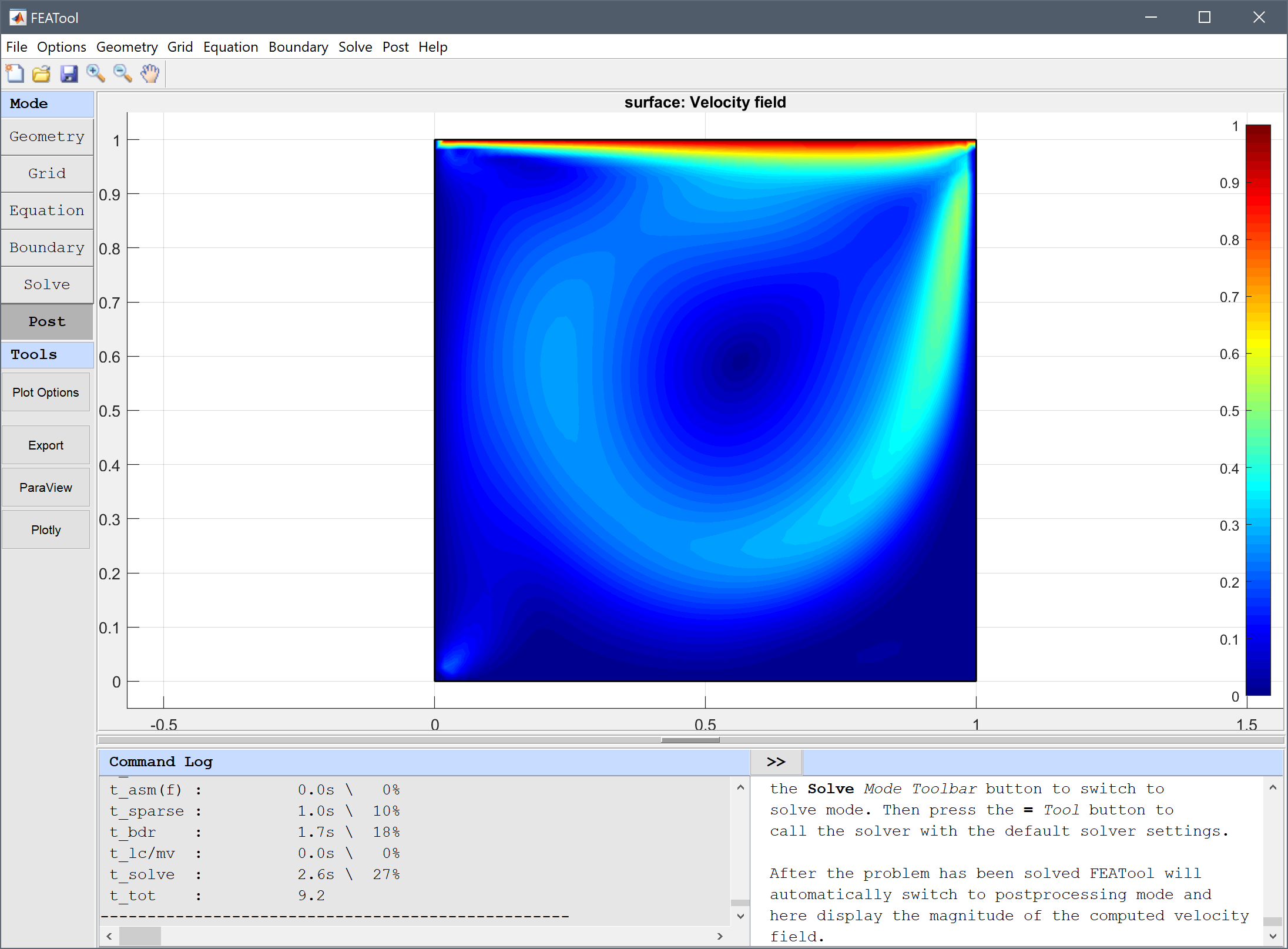
After the problem has been solved FEATool will automatically switch to postprocessing mode and here display the magnitude of the computed velocity field.

1. Press the Plot Options Toolbar button.
2. Select Vorticity from the Predefined surface plot expressions drop-down menu.
3. Select the Contour Plot check box.
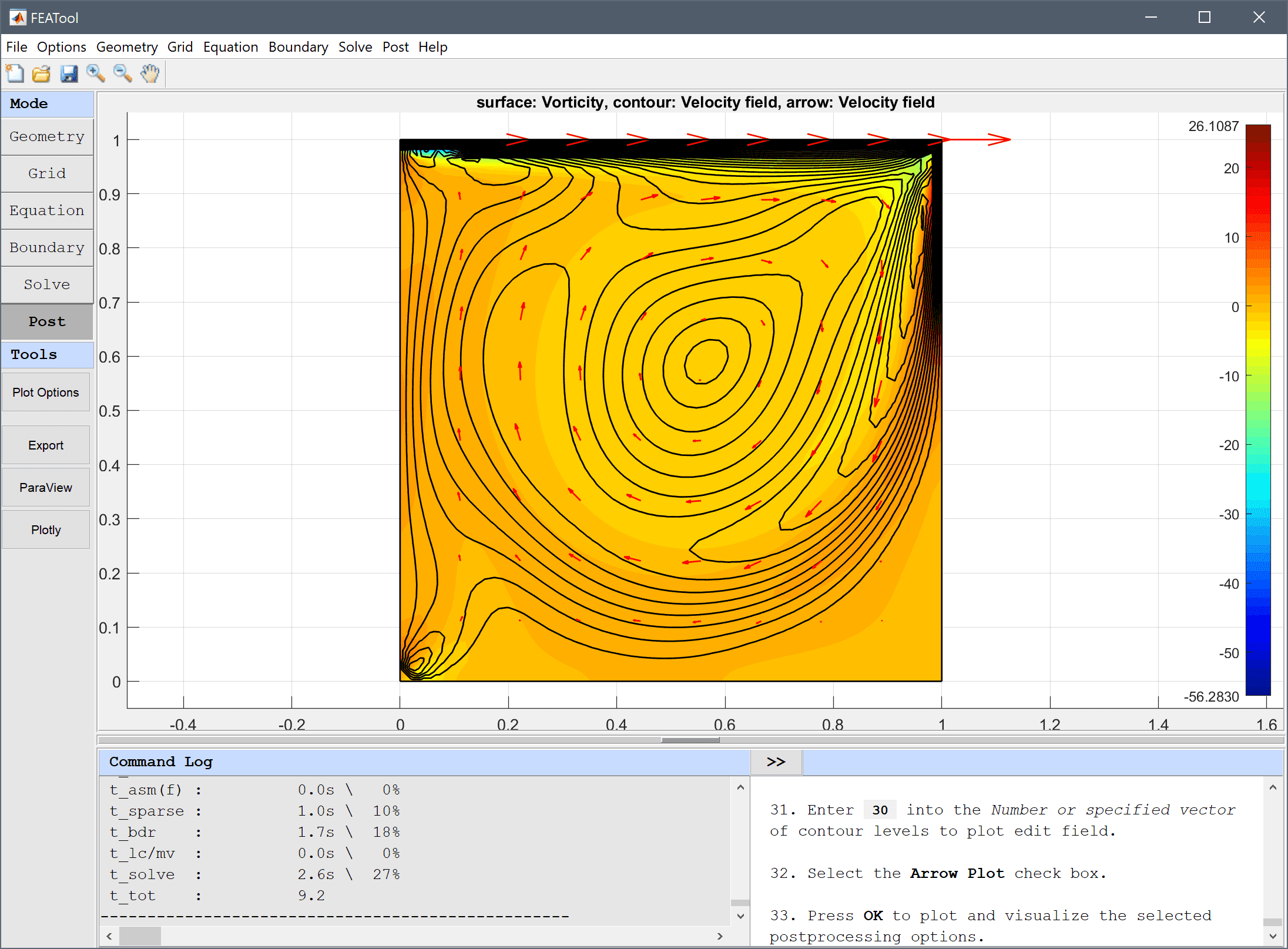
4. Enter 30 into the Number or specified vector of contour levels to plot edit field.
5. Select the Arrow Plot check box.

6. Press OK to plot and visualize the selected postprocessing options.

   

To evaluate the accuracy of the solution the vorticity at (0.53, 0.56) is evaluated. Either click directly at this point or use the Point/Line Evaluation functionality.

1. Select Point/Line Evaluation... from the Post menu.
2. Select Vorticity from the Evaluation Expression drop-down menu.
3. Enter 0.53 into the Evaluation coordinates in x-direction edit field.

4. Enter 0.564 into the Evaluation coordinates in y-direction edit field.

   

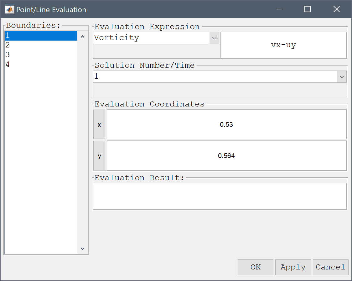
5. Press OK to finish and close the dialog box.

   

The computed vorticity at the evaluated point is -1.73 which is quite close to the reference value of -2.068, to achieve a better approximation a finer grid and higher order discretization would be necessary.

The flow in driven cavity fluid dynamics model has now been completed and can be saved as a binary (.fea) model file, or exported as a programmable MATLAB m-script text file (available as the example ex_navierstokes2 script file), or GUI script (.fes) file.

References

[1] Botella O, Peyret R. Benchmark spectral results on the lid-driven cavity flow. Computers and Fluids 27(4):421-433, 1998.

[2] Erturk E, Corke TC, Gokcol C. Numerical solutions of 2-D steady incompressible driven cavity flow at high Reynolds numbers. Int- ernational Journal for Numerical Methods in Fluids 37(6):633-655, 2005.

[3] Nishida H, Satofuka N. Higher-order solutions of square driven cavity flow using a variable-order multi-grid method. International Journal for Numerical Methods in Engineering 34(2):637-653, 1992.

[4] Schreiber R, Keller HB. Driven cavity flows by efficient numerical techniques. Journal of Computational Physics 49(2):310-333, 1983.