|
|
FEATool Multiphysics
v1.18.0
Finite Element Analysis Toolbox
|
|
|
FEATool Multiphysics
v1.18.0
Finite Element Analysis Toolbox
|
A well known benchmark, test, and validation problem suite for incompressible fluid flows are the DFG cylinder benchmark problems. Although it is not possible to derive analytical solutions to these test cases, accurate numerical solutions to benchmark reference quantities have been established for a number of configurations [1], [2].
The test configuration used in the following places a solid cylinder centered at (0.2, 0.2) with diameter \(D=0.1\) in a \(L=2.2\) by \(H=0.41\) rectangular channel. The fluid density \(\rho\) is taken as 1 and the viscosity \(\mu\) is 0.001. A fully developed parabolic velocity profile is prescribed at the inlet, \(\mathbf{u}_{inflow} = \mathbf{u}(0, y) = 4U_{max}H^{-2}(y(H-y), 0)\), with the maximum velocity \(U_{max}=0.3\). This results in a mean velocity \(U_{mean}=0.2\) and a Reynolds number \(Re=\rho U_{mean}D/\mu=20\) and thus the flow field will be laminar.
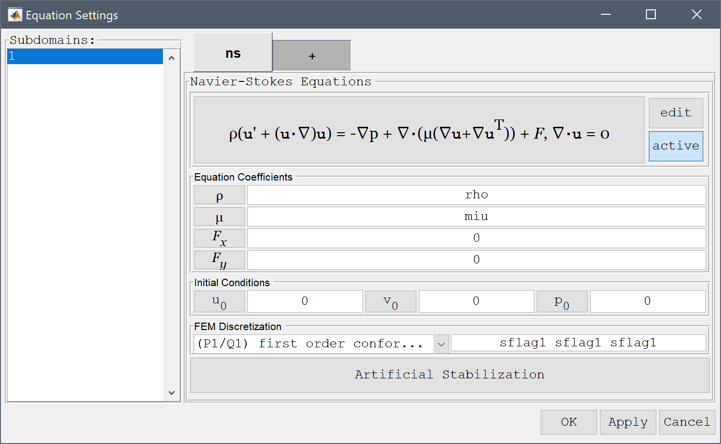
As the fluid is considered incompressible the problem is governed by the Navier-Stokes equations. That is,
\[ \left\{\begin{aligned} \rho\left( \frac{\partial\mathbf{u}}{\partial t} + (\mathbf{u}\cdot\nabla)\mathbf{u}\right) - \nabla\cdot(\mu(\nabla\mathbf{u}+\nabla\mathbf{u}^T)) + p &= \mathbf{F} \\ \nabla\cdot\mathbf{u} &= 0 \end{aligned}\right. \]
where in this case the time dependent term can be neglected. The benchmark quantities that should be computed include the pressure difference between the front and rear of the cylinder \(\Delta p = p(0.15,0.2)−-p(0.25,0.2)\), and the coefficients of drag \(c_d\) and lift \(c_l\), defined as
\[ c_d = \frac{2F_d}{\rho U_{mean}^2 D},\qquad c_l = \frac{2F_l}{\rho U_{mean}^2 D} \]
The drag and lift forces, \(F_d\) and \(F_l\), can be computed as
\[ F_d = \phantom{-}\int_S \left( \mu\frac{\partial\mathbf{u}_{\tau}(t)}{\partial n}n_y-pn_x \right) dS,\qquad F_l = -\int_S \left( \mu\frac{\partial\mathbf{u}_{\tau}(t)}{\partial n}n_x+pn_y \right) dS \]
where \(\mathbf{u}_{\tau}\) is the velocity in the tangential direction \(\tau = (n_y, -n_x, 0)^T\).
This model is available as an automated tutorial by selecting Model Examples and Tutorials... > Fluid Dynamics > Flow Around a Cylinder from the File menu, viewed as a video tutorial, or alternatively, follow the step-by-step instructions below.
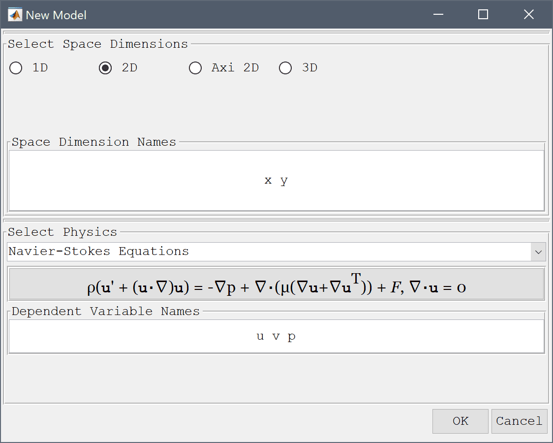
Select the Navier-Stokes Equations physics mode from the Select Physics drop-down menu.
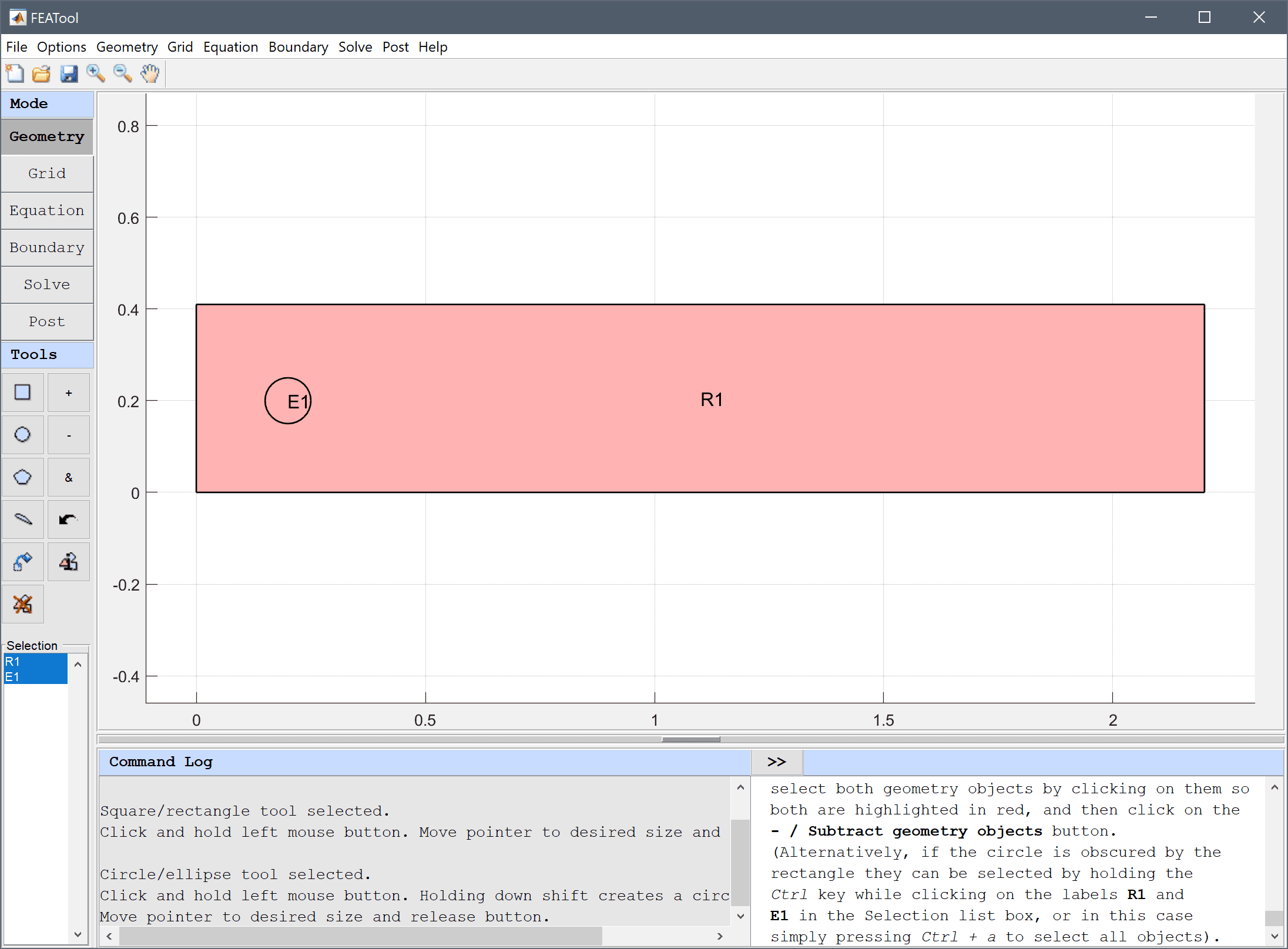
To create a rectangle, first click on the Create square/rectangle Toolbar button. Then left click in the main plot axes window, and hold down the mouse button. Move the mouse pointer to draw the shape outline, and release the button to finalize the shape.
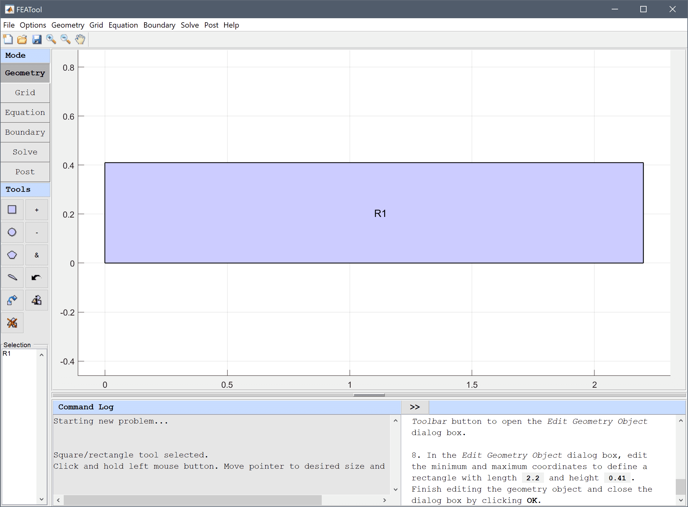
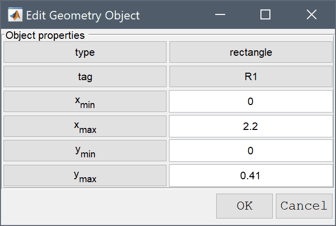
In the Edit Geometry Object dialog box, edit the minimum and maximum coordinates to define a rectangle with length 2.2 and height 0.41. Finish editing the geometry object and close the dialog box by clicking OK.
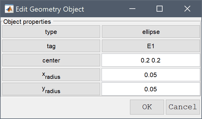
In the Edit Geometry Object dialog box change the center coordinates to 0.2 0.2, and the x and y radius 0.05 in the corresponding edit fields. Finish editing E1 and close the dialog box by clicking OK.
To subtract the circle from the rectangle first select both geometry objects by clicking on them so both are highlighted in red, and then click on the - / Subtract geometry objects button. (Alternatively, if the circle is obscured by the rectangle they can be selected by holding the Ctrl key while clicking on the labels R1 and E1 in the Selection list box, or in this case simply pressing Ctrl + A to select all objects).
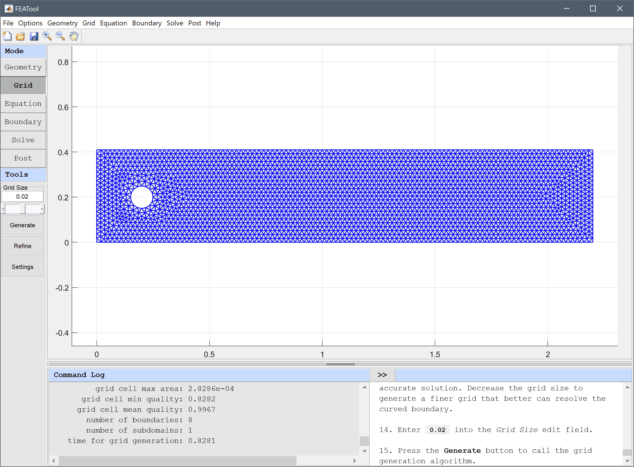
The default grid may be too coarse to ensure an accurate solution. Decrease the grid size to generate a finer grid that better can resolve the curved boundary.
Enter 0.02 into the Grid Size edit field, and press the Generate button to call the grid generation algorithm.
In the Equation Settings dialog box that automatically opens, set the density to 1 and viscosity to 0.001 in the corresponding edit fields. The other coefficients can be left to their zero default values. Press OK to finish and close the dialog box.
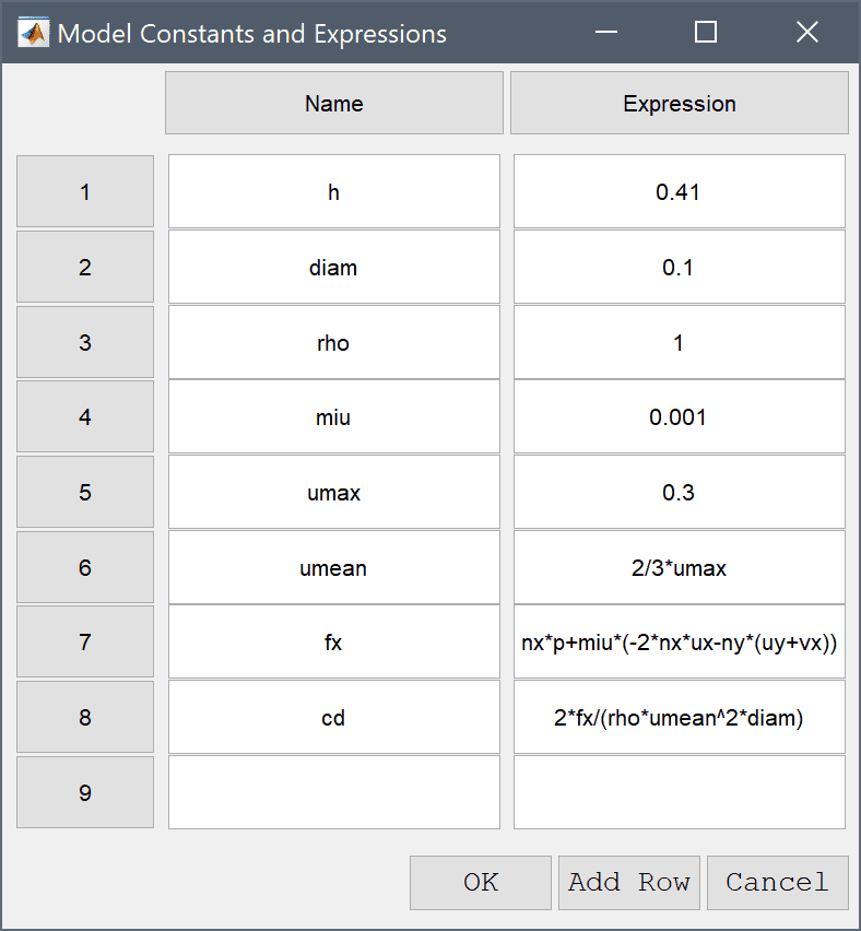
| Name | Expression |
|---|---|
| h | 0.41 |
| diam | 0.1 |
| rho | 1 |
| miu | 0.001 |
| umax | 0.3 |
| umean | 2/3*umax |
| fx | nx*p+miu*(-2*nx*ux-ny*(uy+vx)) |
| cd | 2*fx/(rho*umean^2*diam) |
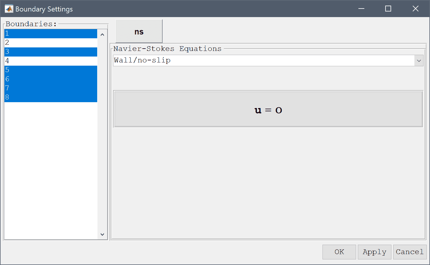
In the Boundary Settings dialog box, first select all boundaries except for the right outflow and left inflow (numbers 1, 3, and 5-8) in the left hand side Boundaries selection list box, and select the Wall/no-slip boundary condition from the drop-down menu.
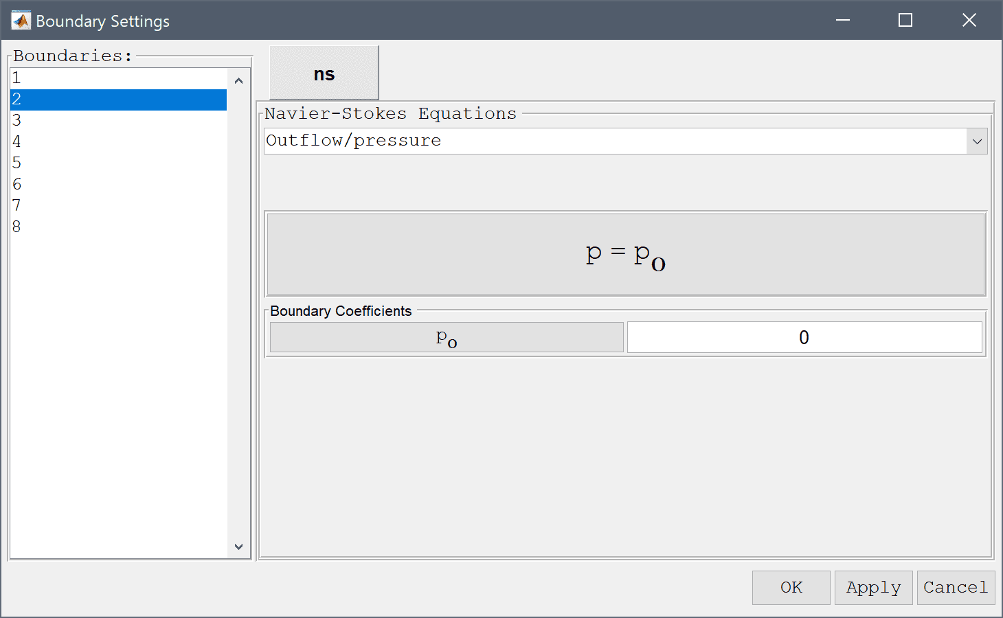
Select the right outflow boundary (number 2) and select the Outflow/pressure boundary condition from the drop-down menu (alternatively one can prescribe the Neutral outflow/stress boundary condition).
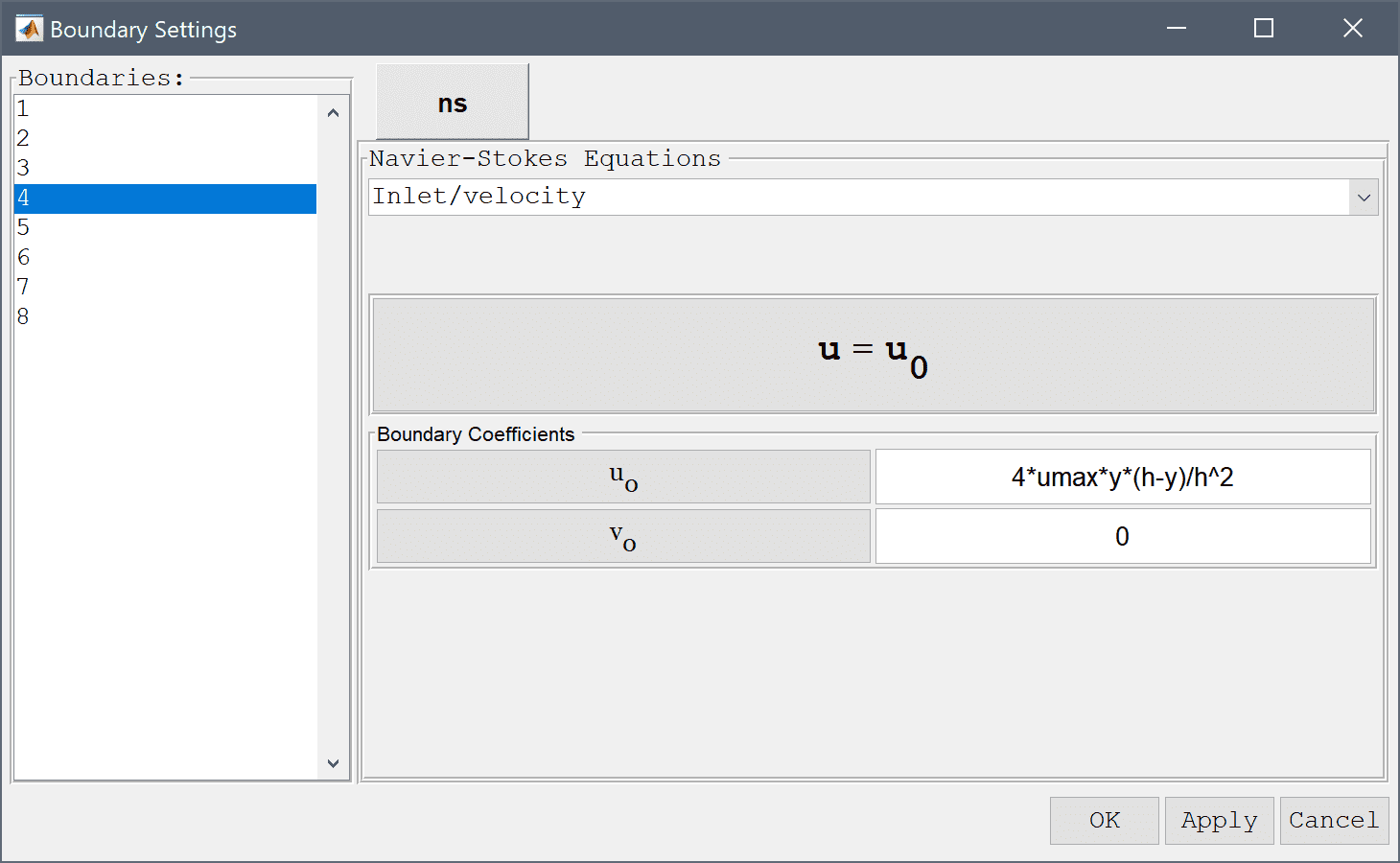
Lastly select the left inflow boundary (number 4) and select the Inlet/velocity boundary condition from the drop-down menu. To specify a parabolic velocity profile enter the expression 4*umax*y*(h-y)/h^2 in the edit field for the velocity coefficient in the x-direction, u0. Press OK to finish the boundary condition specification.
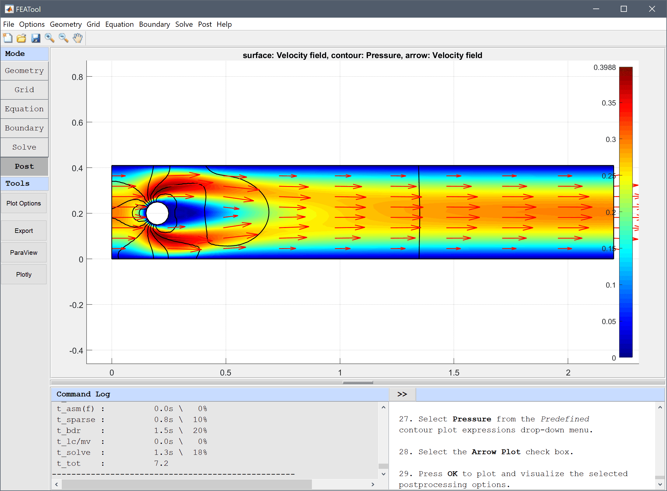
After the problem has been solved FEATool will automatically switch to postprocessing mode and display the computed velocity field.
Select the Arrow Plot check box.
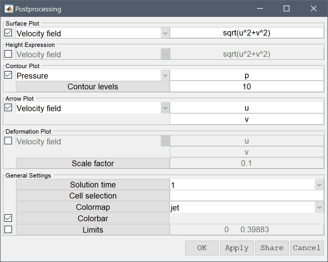
Press OK to plot and visualize the selected postprocessing options.
To calculate the drag coefficient. Select Boundary Integration... from the Post menu. In the Boundary Integration dialog box, select the boundaries which make up the circle (numbers 5-8) in the left hand side Boundaries selection list box. Then enter the name for the previously defined expression for the drag coefficient, cd, in to the Integration Expression edit field. Press the OK or Apply button to show the result in the lower Integration Result frame as well as in the Command Log message window.
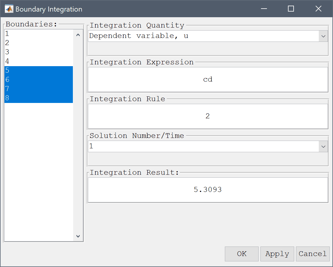
The computed drag coefficient is 5.3 which is close to the reference value of 5.5795. To get a closer result one could use a finer grid along the cylinder boundary, as well as higher order elements which yield higher accuracy for quantities involving derivatives (as the force terms here do).
Similar to the drag one can compute the lift coefficient defining fy as ny*p+miu*(-nx*(uy+vx)-2*ny*vy), and cl = 2*fy/(rho*umean^2*diam). And the pressure difference can be computed by directly evaluating the pressure at the front and back of the cylinder with the Point/Line Evaluation functionality, and computing the difference.
The flow around a cylinder fluid dynamics model has now been completed and can be saved as a binary (.fea) model file, or exported as a programmable MATLAB m-script text file (available as the example ex_navierstokes3 script file), or GUI script (.fes) file.
In addition to the stationary test case described above. An instationary benchmark test case is also available (ex_navierstokes6). This test case uses the same geometry but instead applies an inflow condition that varies with time uinflow = 6·sin(π·t/8)·(y·(0.41-y))/0.412 so that 0 < Re(t) < 100 [3]. Computations with FEATool show that the drag and lift coefficients, and pressure difference between front and rear of the cylinder agree very well with the reference values [4].
[1] Nabh G. On higher order methods for the stationary incompressible Navier-Stokes equations. PhD Thesis, Universität Heidelberg, Preprint 42/98, 1998.
[2] John V, Matthies G. Higher-order finite element discretizations in a benchmark problem for incompressible flows. International Journal for Numerical Methods in Fluids, 37(8):885–903, 2001.
[3] John V. Reference values for drag and lift of a two-dimensional time-dependent flow around a cylinder. International Journal for Numerical Methods in Fluids, 44:777-788, 2004.
[4] John V, Rang J. Adaptive time step control for the incompressible Navier–Stokes equations. Comput. Methods Appl. Mech. Engrg. 199 (2010) 514–524.