Flow over a backwards facing step is a classic computational fluid dynamics test problem which is used extensively for validation of simulation codes. The test problem essentially consists of studying how a fully developed flow profile reacts to a sudden expansion in a channel. The expansion will cause a break in the flow and a recirculation or separation zone will form. To measure and compare results the resulting length of the recirculation or separation zone is used.

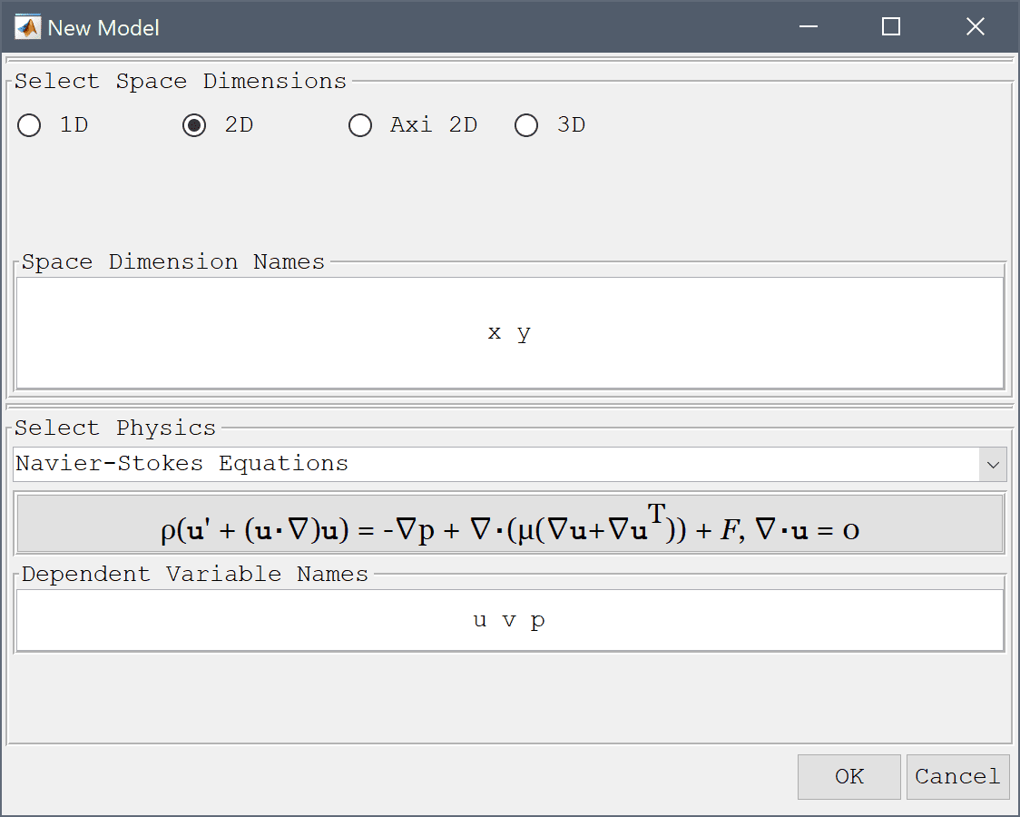
The stationary incompressible Navier-Stokes equations are applied with simulation parameters corresponding to a Reynolds number, Re = 389. The inlet velocity is given as u_inlet = 4u_max (y-h_step)(1-y)/h_inlet² where h_inlet is the channel height, hstep the expansion step height, and u_max = 1 the maximum velocity. No-slip zero velocity conditions are applied to all solid walls, and a suitable outflow condition must also be applied. The reference recirculation zone length found in the references [1,2] is estimated to be 7.93 length units (fraction of the step height).

Tutorial

This model is available as an automated tutorial by selecting Model Examples and Tutorials... > Fluid Dynamics > Flow Over a Backwards Facing Step from the File menu. Or alternatively, follow the step-by-step instructions below. Note that the CFDTool interface differ slightly from the FEATool Multiphysics instructions described in the following.

To start a new model click the New Model toolbar button, or select New Model... from the File menu.
Select the 2D radio button.
Select the Navier-Stokes Equations physics mode from the Select Physics drop-down menu. (Note that for CFDTool the physics selection is done in the Equation settings dialog box.)
Press OK to finish the physics mode selection.
To create a rectangle, first click on the Create square/rectangle Toolbar button. Then left click in the main plot axes window, and hold down the mouse button. Move the mouse pointer to draw the shape outline, and release the button to finalize the shape.

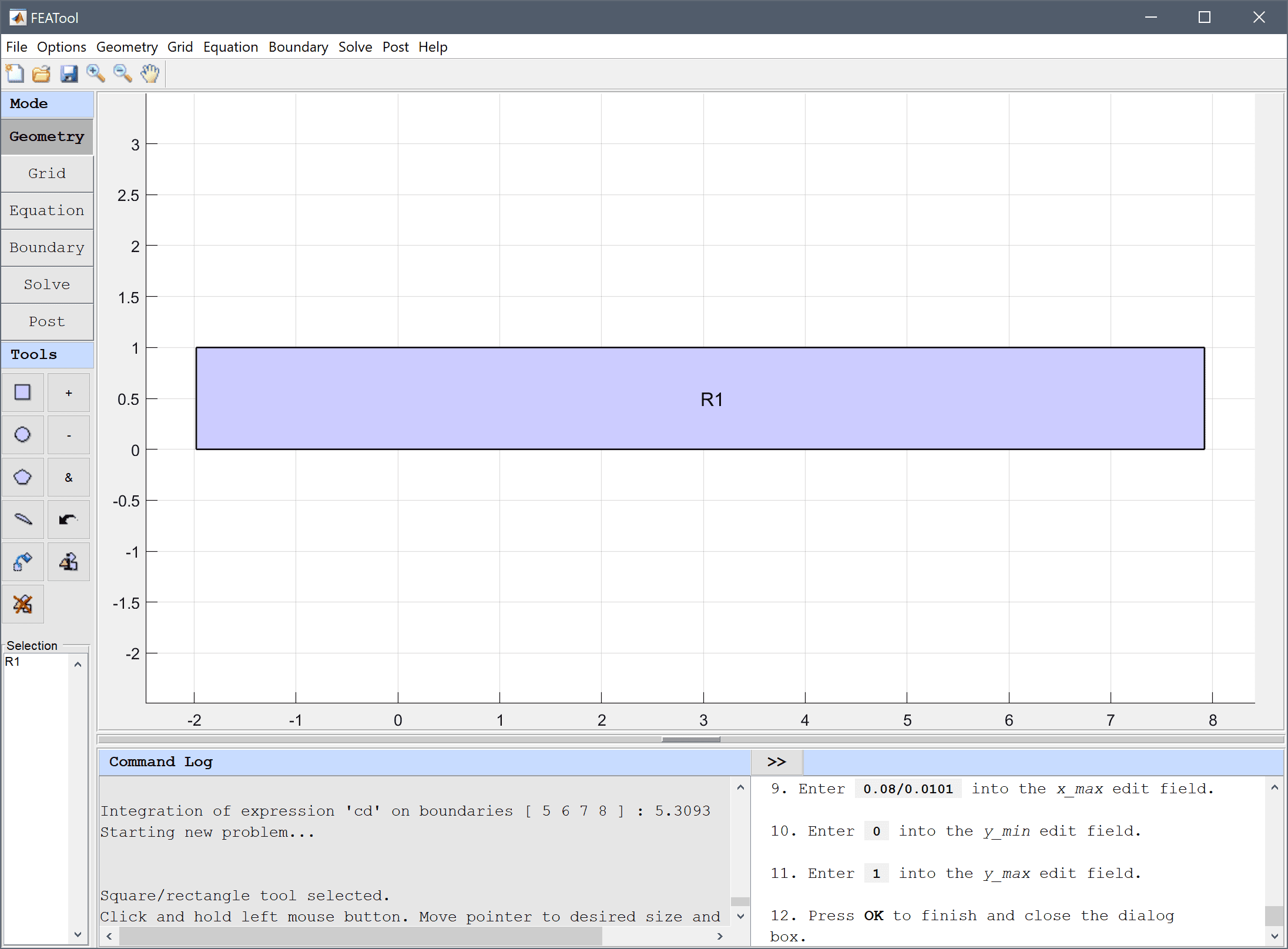
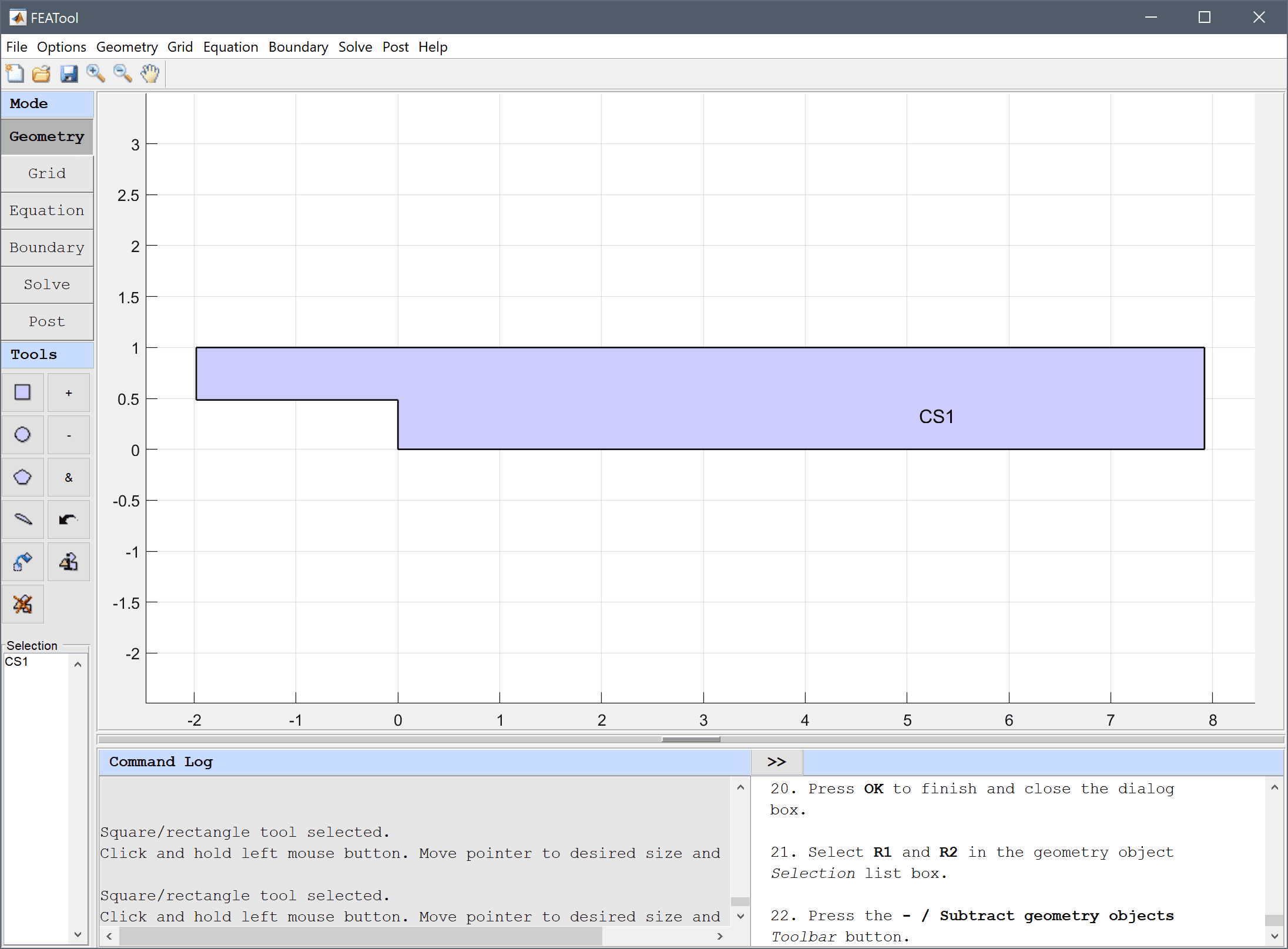
The backwards facing step geometry is generated by creating a larger rectangle for the channel from which a smaller section is removed to create the expansion step. Alternatively, the geometry could also be created by joining two rectangle slices, or directly using the Polygon tool.

First create the outer rectangle with the scaled dimensions 1/0.0101 by 1, with the expansion step located at x = 0.

Select R1 in the geometry object Selection list box.
To modify and edit the selected rectangle, click on the Inspect/edit selected geometry object Toolbar button to open the Edit Geometry Object dialog box.
Enter -0.02/0.0101 into the x_min edit field.
Enter 0.08/0.0101 into the x_max edit field.
Enter 0 into the y_min edit field.
Enter 1 into the y_max edit field.
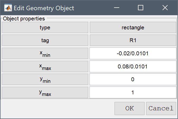
Press OK to finish and close the dialog box.

Then create and subtract a second smaller rectangle with dimensions 1.9802 by 0.0049/0.0101 to create the step.

To create a rectangle, first click on the Create square/rectangle Toolbar button. Then left click in the main plot axes window, and hold down the mouse button. Move the mouse pointer to draw the shape outline, and release the button to finalize the shape.
Select R2 in the geometry object Selection list box.
To modify and edit the selected rectangle, click on the Inspect/edit selected geometry object Toolbar button to open the Edit Geometry Object dialog box.
Enter -0.02/0.0101 into the x_min edit field.
Enter 0 into the x_max edit field.
Enter 0 into the y_min edit field.
Enter 0.0049/0.0101 into the y_max edit field.
Press OK to finish and close the dialog box.
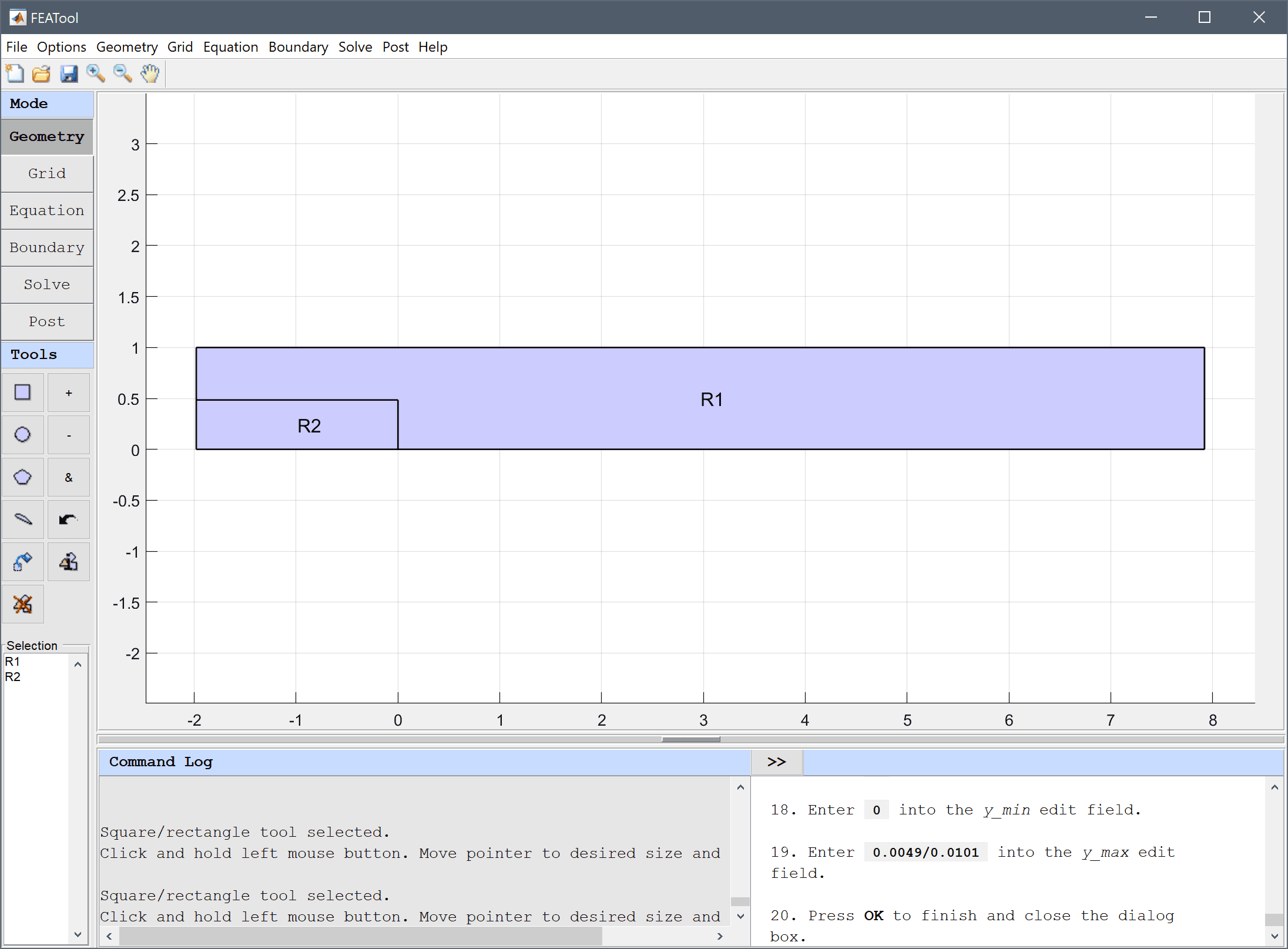
Select R1 and R2 in the geometry object Selection list box.
Press the - / Subtract geometry objects Toolbar button.
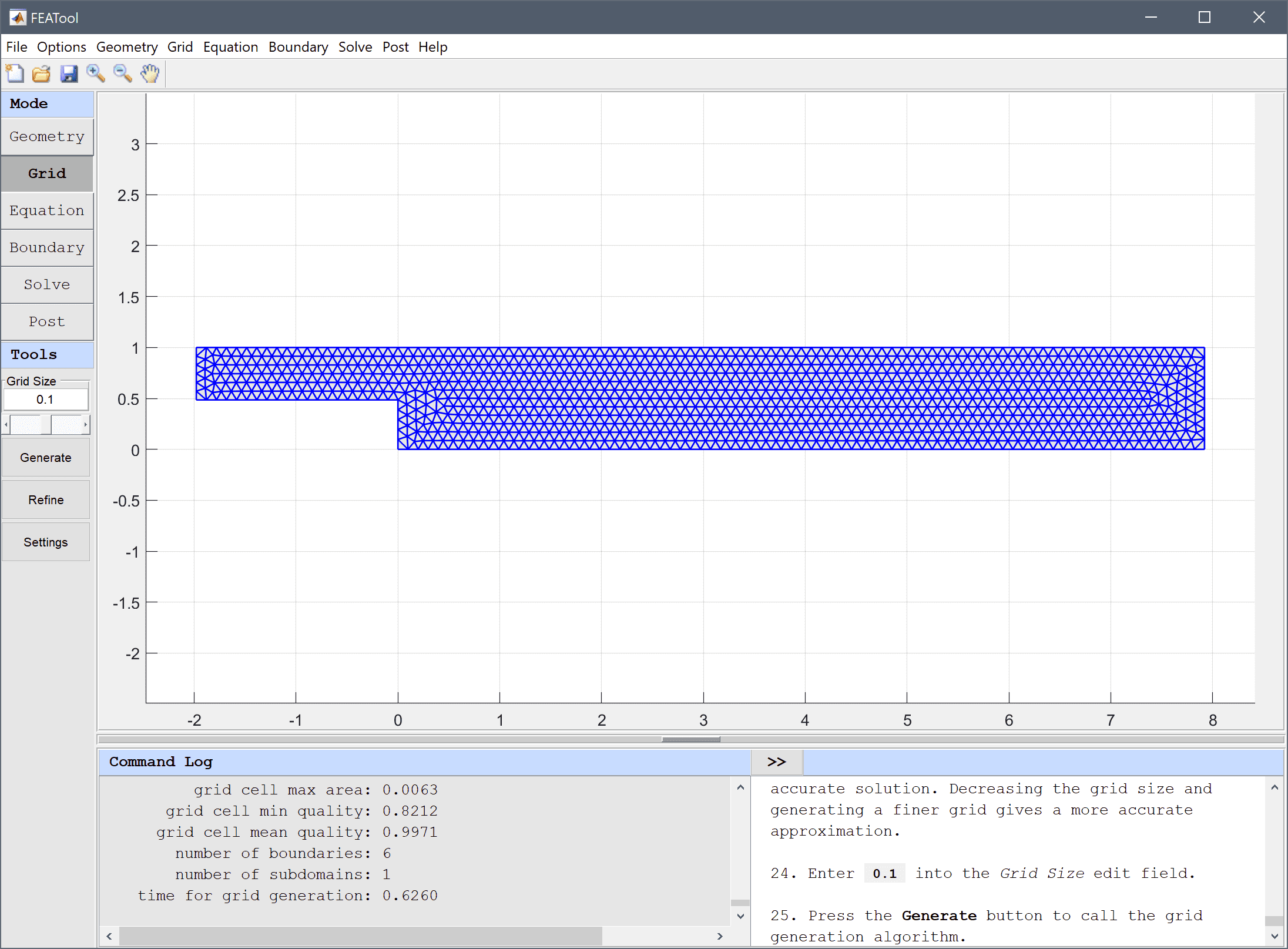
Switch to Grid mode by clicking on the corresponding Mode Toolbar button.

The default grid may be too coarse to ensure an accurate solution. Decreasing the grid size and generating a finer grid gives a more accurate approximation.

Enter 0.1 into the Grid Size edit field.
Press the Generate button to call the grid generation algorithm.
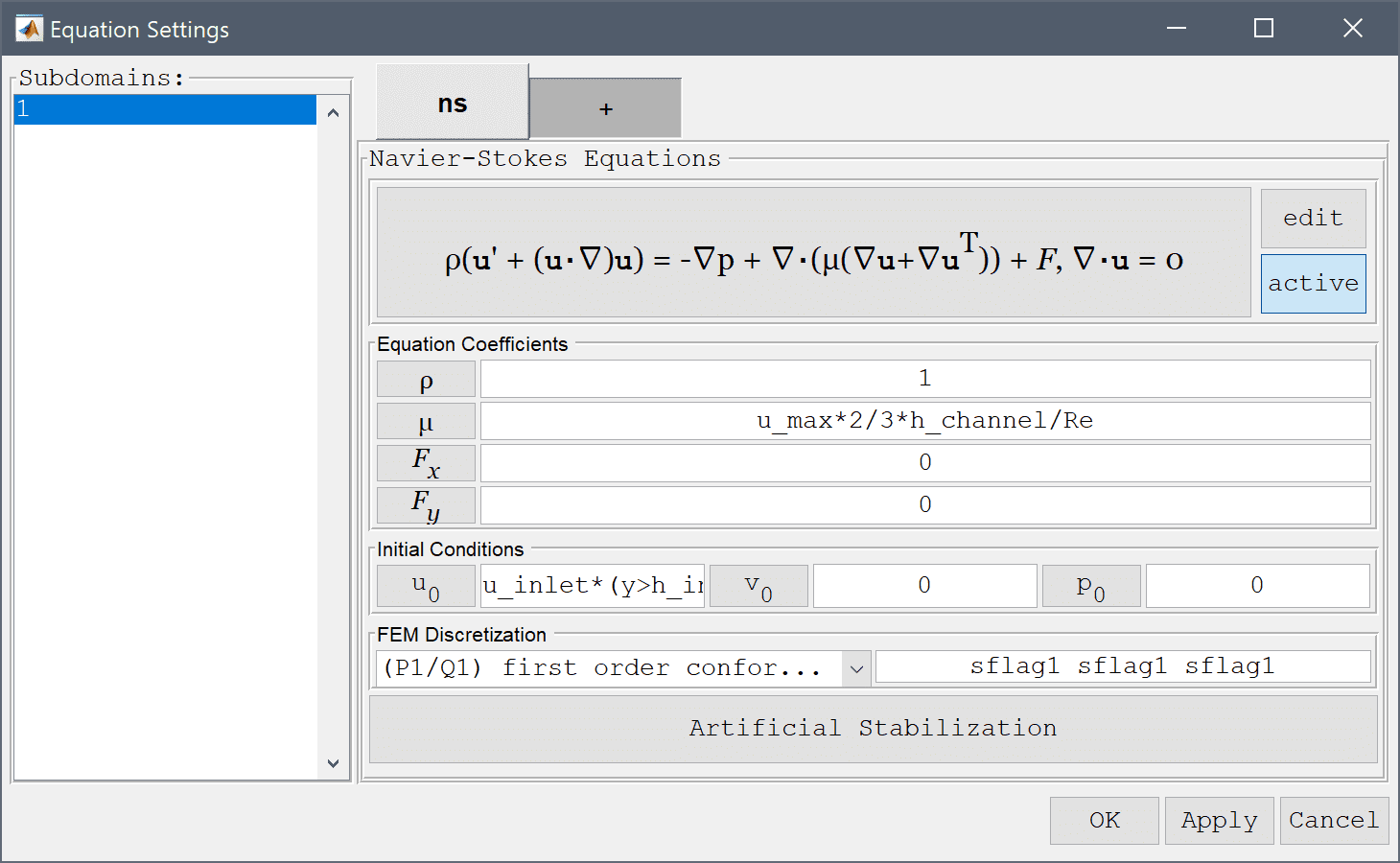
Switch to Equation mode by clicking on the corresponding Mode Toolbar button.
In the Equation Settings dialog box that automatically opens, set the density to 1 and viscosity to u_max*2/3*h_channel/Re in the corresponding edit fields. In order to start with a better initial guess, set the initial condition for the x-velocity u0 to u_inlet*(y>h_inlet). The other coefficients can be left to their default values. Press OK to finish and close the dialog box. (Note that the Equation Settings dialog box may look different for CFDTool.)
Press the Constants Toolbar button, or select the corresponding entry from the Equation menu, to open the Model Constants and Expressions dialog box. Enter the following expressions for the channel, fluid parameters, and inlet velocity expression. Press Enter after the last expression or use the Add Row button to expand the expression list.

Name	Expression
h_step	0.0049/0.0101
h_channel	1
h_inlet	h_channel-h_step
u_max	1
Re	389
u_inlet	4u_max(y-h_step)*(1-y)/h_inlet^2

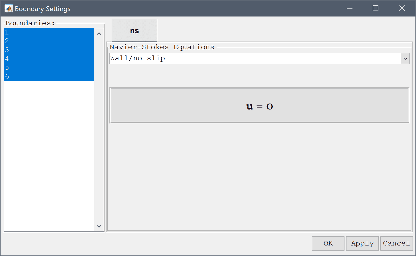
Switch to Boundary mode by clicking on the corresponding Mode Toolbar button.
In the Boundary Settings dialog box, first select all boundaries except for the right outflow and left inflow (numbers 1, 3, and 5-8) in the left hand side Boundaries selection list box, and select the Wall/no-slip boundary condition from the drop-down menu.
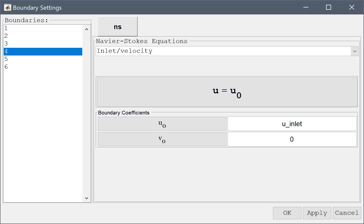
Select the leftmost boundary (number 4) and choose the Inlet/velocity boundary condition from the drop-down menu. When using the default built-in solver enter the previously defined u_inlet expression in the edit field for the x-velocity coefficient u0.
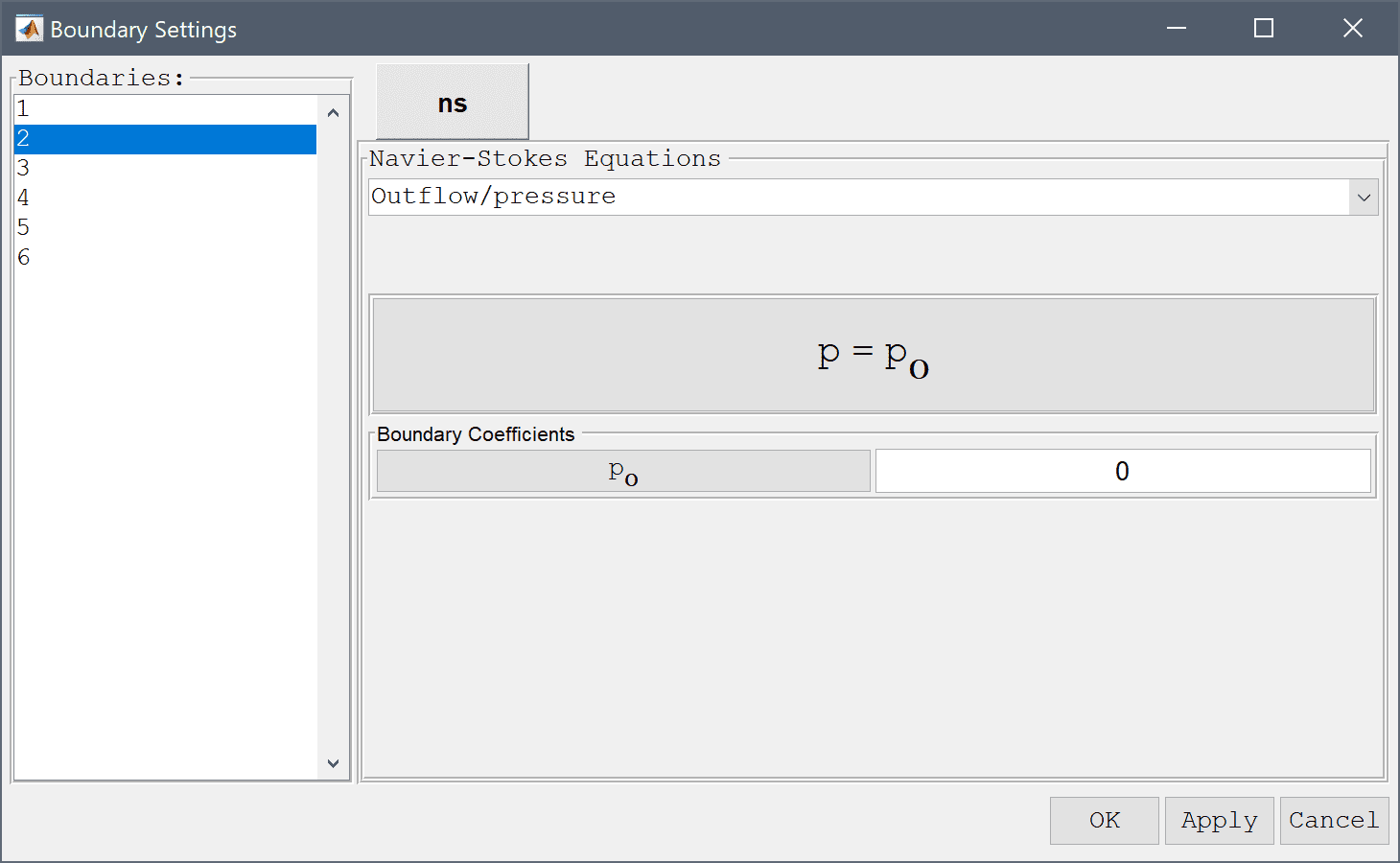
Finally, select the right outflow boundary (number 2) and select the Outflow/pressure boundary condition from the drop-down menu (alternatively one can prescribe the Neutral outflow/stress boundary condition). Finish by clicking the OK button.
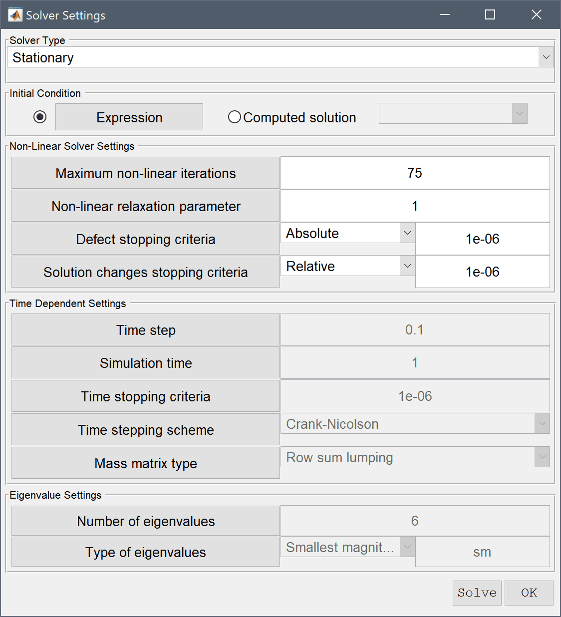
Now that the problem has been defined, press the Solve Mode Toolbar button to switch to solve mode, and press the Settings button to open the Solver Settings dialog box.
In the Solver Settings dialog box increase the Maximum non-linear iterations to 75 in the Non-Linear Solver Settings section to allow for the non-linear problem to converge.
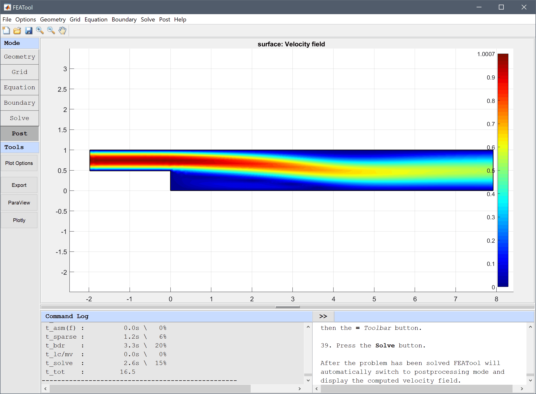
To start the solver with the chosen settings press the Solve button, or press OK and then the = Toolbar button.
Press the Solve button.

After the problem has been solved FEATool will automatically switch to postprocessing mode and display the computed velocity field.

To see the recirculation zone clearer, open the Postprocessing settings dialog box and enter the expression for the normalized recirculation zone length x/h_step*(u<0)*(y<h_step) in the Surface Plot expression edit field (Note that switch type expressions such as a<b evaluate to either 0 or 1, and are used here to limit the plot to the lower half region for which the u velocity is negative). The Arrow Plot option can also be used to help visualize the flow field.

Press the Plot Options Toolbar button.
Enter x/h_step*(u<0)*(y<h_step) into the User defined surface plot expression edit field.
Press OK to plot and visualize the selected postprocessing options.

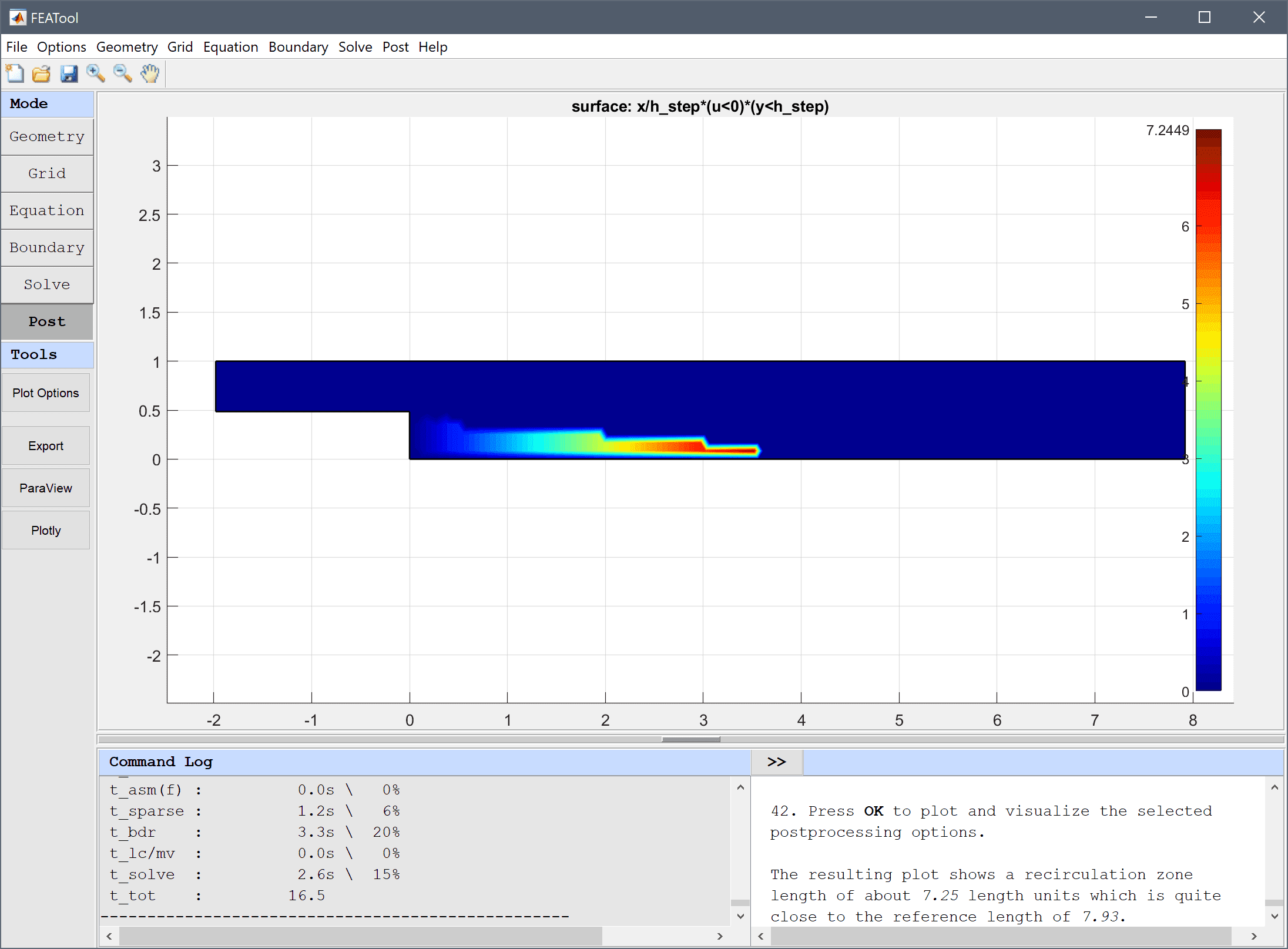
The resulting plot shows a recirculation zone length of about 7.25 length units which is in the same range as the reference length of 7.93.

The flow over a backwards facing step fluid dynamics model has now been completed and can be saved as a binary (.fea) model file, or exported as a programmable MATLAB m-script text file (available as the example ex_navierstokes4 script file), or GUI script (.fes) file.

References

[1] Gresho PM, Sani RL. Incompressible Flow and the Finite Element Method. Volume 1 & 2, John Wiley & Sons, New York, 2000.

[2] Rose A, Simpson B. Laminar, Constant-Temperature Flow Over a Backward Facing Step. 1st NAFEMS Workbook of CFD Examples, Glasgow, UK, 2000.