Vortex Flow

Time dependent decaying flow for standing vortices with the following analytical solution to the Navier-Stokes equations

\[ \left\{\begin{array}{l} u = -cos(kx) sin(ky) e^{-2\nu k^2t} \\ v = sin(kx) cos(ky) e^{-2\nu k^2 t} \\ p = -\frac{1}{4}(cos(2kx)+cos(2ky)) e^{-4\nu k^2 t} \end{array}\right. \]

The two-dimensional flow problem is solved for a unit square with k = 2π and the exact solution as boundary and initial conditions.

Tutorial

This model is available as an automated tutorial by selecting Model Examples and Tutorials... > Fluid Dynamics > Vortex Flow from the File menu. Or alternatively, follow the step-by-step instructions below.

1. To start a new model click the New Model toolbar button, or select New Model... from the File menu.
2. Select the 2D radio button.
3. Select the Navier-Stokes Equations physics mode from the Select Physics drop-down menu.
4. Press OK to finish the physics mode selection.
5. To create a rectangle, first click on the Create square/rectangle Toolbar button. Then left click in the main plot axes window, and hold down the mouse button. Move the mouse pointer to draw the shape outline, and release the button to finalize the shape.
6. Select R1 in the geometry object Selection list box.
7. To modify and edit the selected rectangle, click on the Inspect/edit selected geometry object Toolbar button to open the Edit Geometry Object dialog box.
8. Enter 0 into the x_min edit field.
9. Enter 1 into the x_max edit field.
10. Enter 0 into the y_min edit field.
11. Enter 1 into the y_max edit field.
12. Press OK to finish and close the dialog box.
13. Switch to Grid mode by clicking on the corresponding Mode Toolbar button.
14. Enter 0.05 into the Grid Size edit field.
15. Press the Generate button to call the grid generation algorithm.
16. Switch to Equation mode by clicking on the corresponding Mode Toolbar button.
17. Press the Constants Toolbar button, or select the corresponding entry from the Equation menu, to open the Model Constants and Expressions dialog box. Enter the following expressions for the viscosity, vortex period, and reference solutions.

Name	Expression
nu	0.0.1
k	2*pi
u_ref	-cos(k*x)*sin(k*y)*exp(-2*nu*k^2*t)
v_ref	sin(k*x)*cos(k*y)*exp(-2*nu*k^2*t)
p_ref	-1/4*(cos(2*k*x)+cos(2*k*y))*exp(-4*nu*k^2*t)

Open the Equation Settings dialog box and enter nu for the viscosity and the reference expressions as initial conditions

1. Select Equation Settings... from the Equation menu.
2. Enter nu into the Viscosity edit field.
3. Enter u_ref into the Initial condition for u edit field.
4. Enter v_ref into the Initial condition for v edit field.
5. Enter p_ref into the Initial condition for p edit field.
6. Press OK to finish the equation and subdomain settings specification.
7. Switch to Boundary mode by clicking on the corresponding Mode Toolbar button.

Prescribe the reference velocities on all boundaries using the Inlet/velocity boundary condition.

1. Select 1, 2, 3, and 4 in the Boundaries list box.
2. Select Inlet/velocity from the Navier-Stokes Equations drop-down menu.
3. Enter u_ref into the Velocity in x-direction edit field.
4. Enter v_ref into the Velocity in y-direction edit field.
5. Press OK to finish the boundary condition specification.

Also prescribe the reference pressure on all four points. Note that since no outflow is present in this model, a reference point with pressure p = 0 has already been prescribed. This is necessary to ensure convergence and a unique pressure for stationary problems without any outflow boundary conditions.

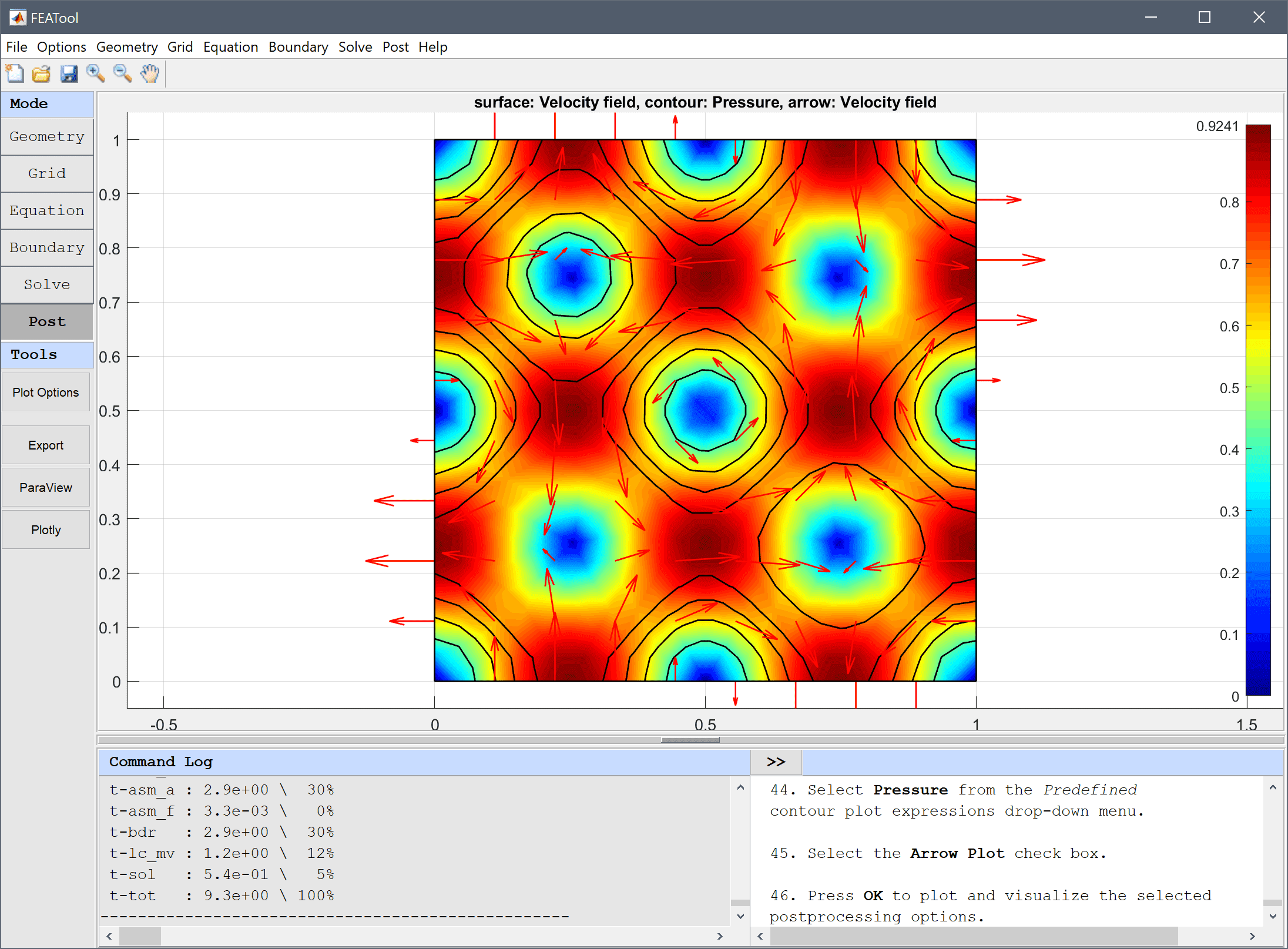
1. Select Add Point Constraints... from the Boundary menu.
2. Enter p_ref into the four edit fields for the corners corresponding to the pressure.
3. Press OK to finish and close the dialog box.
4. Switch to Solve mode by clicking on the corresponding Mode Toolbar button.
5. Press the Settings Toolbar button.
6. Select Time-Dependent from the Solution and solver type drop-down menu.
7. Enter 0.01 into the Time step size edit field.
8. Enter 0.1 into the Duration of time-dependent simulation (maximum time) edit field.
9. Press the Solve button.

Plot the velocity field as arrows and pressure as contour plot to see the vortices of the flow field.

1. Press the Plot Options Toolbar button.
2. Select the Contour Plot check box.
3. Select Pressure from the Predefined contour plot expressions drop-down menu.
4. Select the Arrow Plot check box.
5. Press Apply to plot and visualize the selected postprocessing options.

By plotting and visualizing the difference between the computed and reference variables, the overall accuracy of the simulation can be estimated.

1. Enter u-u_ref into the User defined surface plot expression edit field.
2. Press OK to plot and visualize the selected postprocessing options.

The vortex flow fluid dynamics model has now been completed and can be saved as a binary (.fea) model file, or exported as a programmable MATLAB m-script text file (available as the example ex_navierstokes5 script file), or GUI script (.fes) file.