|
|
FEATool Multiphysics
v1.18.0
Finite Element Analysis Toolbox
|
|
|
FEATool Multiphysics
v1.18.0
Finite Element Analysis Toolbox
|
This 2D verification test case studies steady inviscid compressible flow past a wedge at an incident angle of 15 degrees. As the supersonic flow (Ma = 2.5) hits the wedge a sharp oblique shock wave is formed, resulting in a reduced downstream flow velocity. The simulation uses the inviscid compressible Euler equations to model the flow, adaptively refining the mesh, and using FEM-TVD upwinding to stabilize the solution and resolve shock discontinuities [1].
The angle of the shock wave and downstream Mach number can be determined using oblique shock theory, Ma = 1.873526 at an angle of 36.9449 degrees, and also comparing to results from the NASA/NPARC CFD Verification and Validation Database and from the Wind-US CFD code [2].
This model is available as an automated tutorial by selecting Model Examples and Tutorials... > Fluid Dynamics > Supersonic Flow Past a Wedge from the File menu. Or alternatively, follow the step-by-step instructions below.
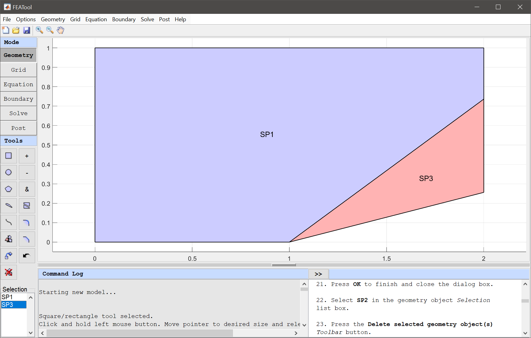
The geometry can be created by splitting a rectangle at the base of the wedge.
0 into the xmin edit field.2 into the xmax edit field.0 into the ymin edit field.1 into the ymax edit field.First split the rectangle at the point (1, 0) at and angle of 15 degrees, and then split again at 15 + 36.9449 degrees (to create an internal edge where the shock will be), then delete the lower segment.
1 0 into the Cutline point edit field.1 atan(pi*15/180) into the Cutline direction vector edit field.1 0 into the Cutline point edit field.1 atan(pi*(15+36.9449)/180) into the Cutline direction vector edit field.Press the Delete selected geometry object(s) Toolbar button.
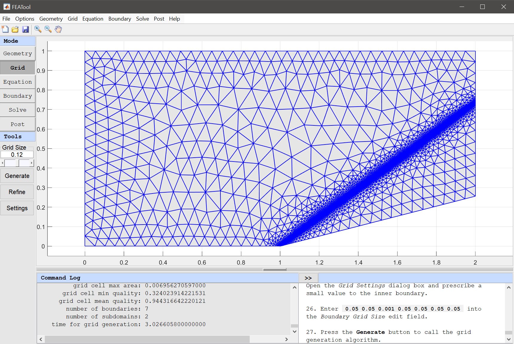
Open the Grid Settings dialog box and prescribe a smaller value to the inner boundary.
0.05 0.05 0.001 0.05 0.05 0.05 0.05 into the Boundary Grid Size edit field.Press OK to finish and close the dialog box.
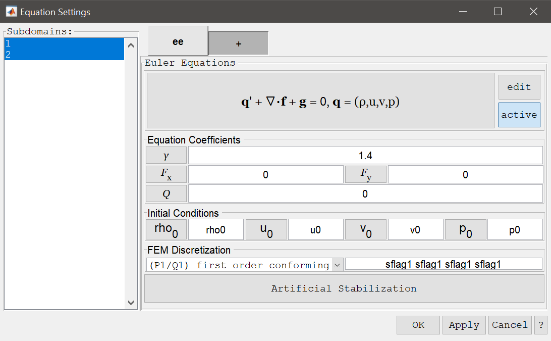
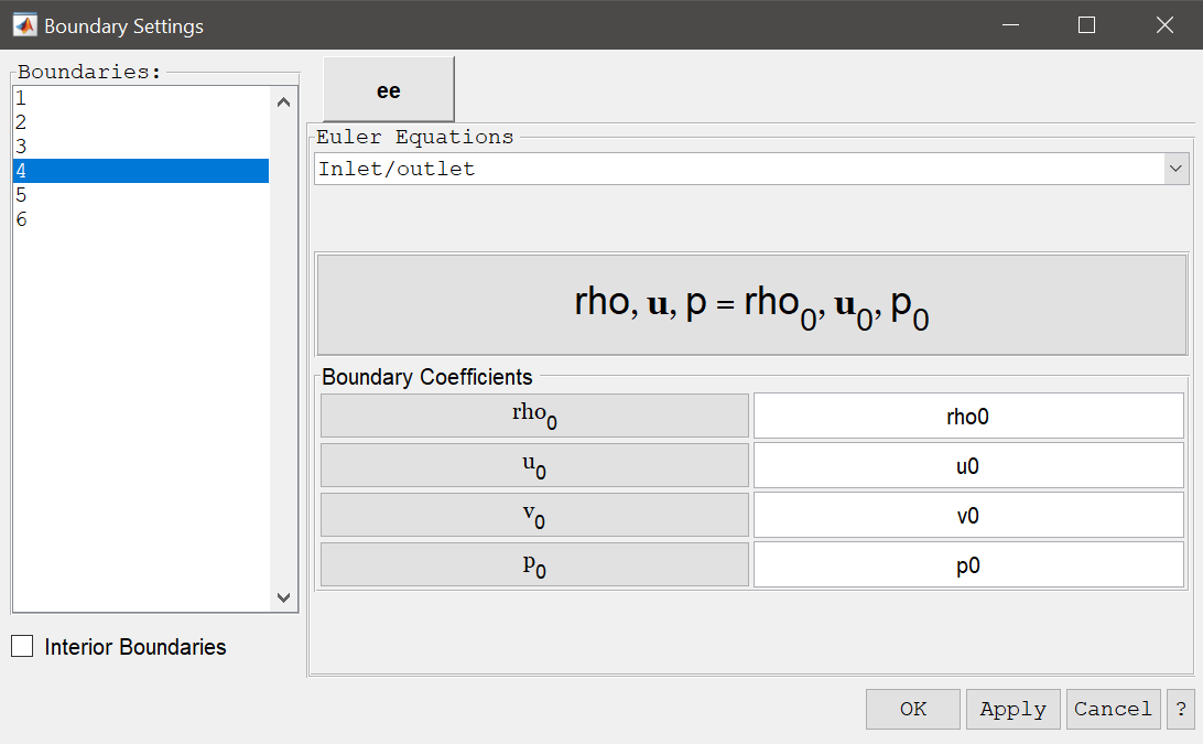
First select both subdomains, and enter placeholder names for the initial flow coefficients.
1.4 into the Ratio of specific heats edit field.rho0 into the Initial condition for rho edit field.u0 into the Initial condition for u edit field.v0 into the Initial condition for v edit field.Enter p0 into the Initial condition for p edit field.
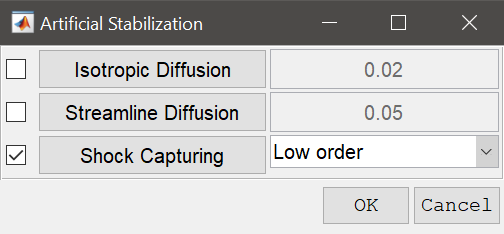
For this problem it is beneficial to use FEM-TVD stablilization (Shock Capturing - Low Order), which ensures that the shock can be captured sharply without unphysical over or under-shoots.
Select the Enable/disable shock capturing check box.
| Name | Expression |
|---|---|
| Ma | 1.4 |
| rho0 | 1 |
| p0 | 1 |
| u0 | Ma*sqrt(1.4*p0/rho0) |
| v0 | 0 |
rho0 into the Density edit field.u0 into the Velocity in x-direction edit field.v0 into the Velocity in y-direction edit field.Enter p0 into the Pressure edit field.
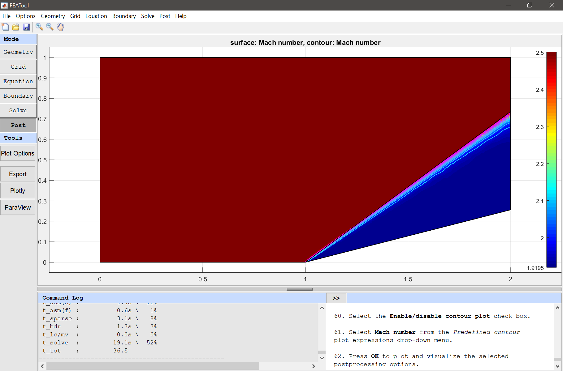
50, and decrease the Non-linear relaxation parameter to 0.9, to allow for the non-linear problem to converge.After the problem has been solved FEATool will automatically switch to postprocessing mode and here display the magnitude of the computed velocity field where the shock pattern can easily be seen. Plot the Mach number and click on a point in the downstream region to verify that the lower Mach number is close to the reference value (1.873526).
Press OK to plot and visualize the selected postprocessing options.
The supersonic flow past a wedge fluid dynamics model has now been completed and can be saved as a binary (.fea) model file, or exported as a programmable MATLAB m-script text file (available as the example ex_compressibleeuler6 script file), or GUI script (.fes) file.
[1] D. Kuzmin, High-resolution FEM-TVD schemes based on a fully multidimensional flux limiter, Journal of Computational Physics, vol. 198, pp. 131-158, 2004.
[2] NPARC Alliance, Computational Fluid Dynamics (CFD) Verification and Validation Web Site.