Turbulent Channel Flow

Simulation of stationary and incompressible turbulent flow between two parallel flat plates at Reynolds number 42800. A fully developed turbulent velocity profile is formed at the outflow boundary which can be compared to experimental results (Laufer, J. 1950).

This example uses both the built-in algebraic mixing length turbulence model, as well as shows how to implement custom user-defined modeling expressions.

Tutorial

This model is available as an automated tutorial by selecting Model Examples and Tutorials... > Fluid Dynamics > Turbulent Channel Flow from the File menu. Or alternatively, follow the step-by-step instructions below.

1. To start a new model click the New Model toolbar button, or select New Model... from the File menu.

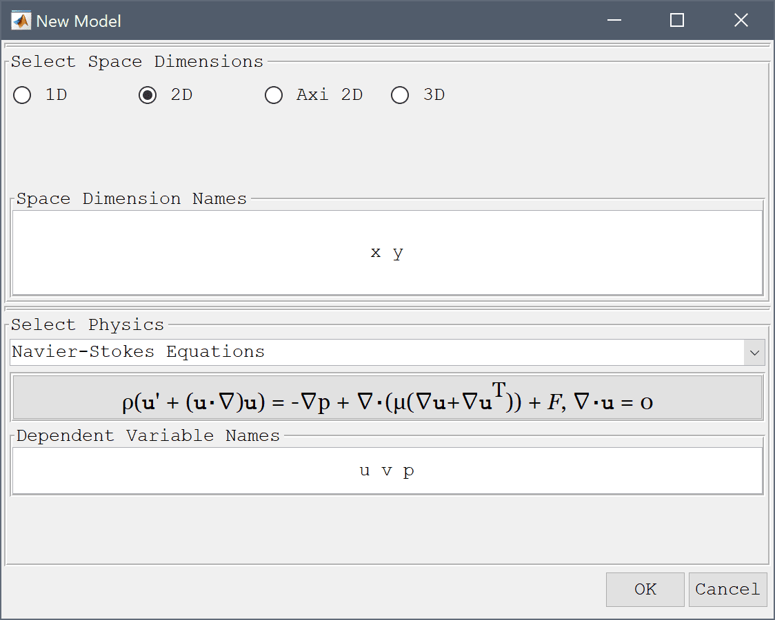
2. Select the Navier-Stokes Equations physics mode from the Select Physics drop-down menu.

   
3. Press OK to finish the physics mode selection.

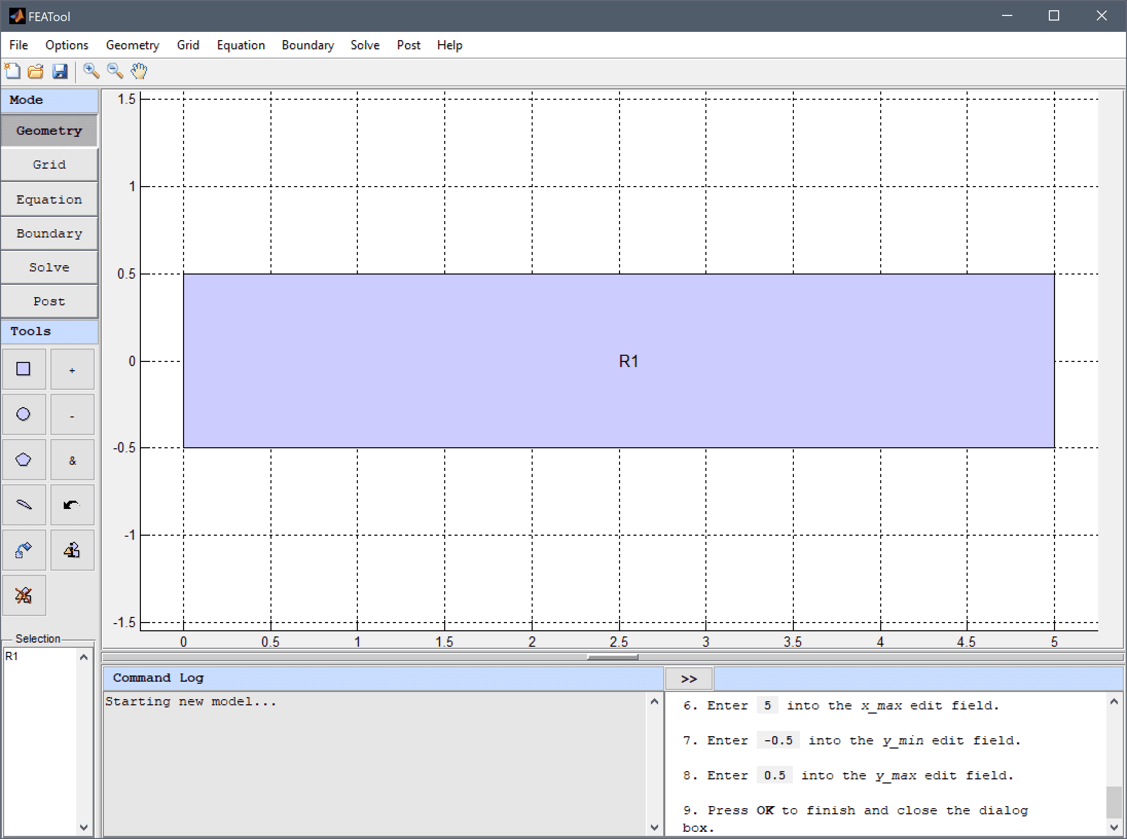
The first step is to create a 1 by 5 rectangle to represent the fluid domain.

1. Select Rectangle from the Geometry menu.
2. Enter 0 into the x_min edit field.
3. Enter 5 into the x_max edit field.
4. Enter -0.5 into the y_min edit field.
5. Enter 0.5 into the y_max edit field.

6. Press OK to finish and close the dialog box.

   
7. Switch to Grid mode by clicking on the corresponding Mode Toolbar button.

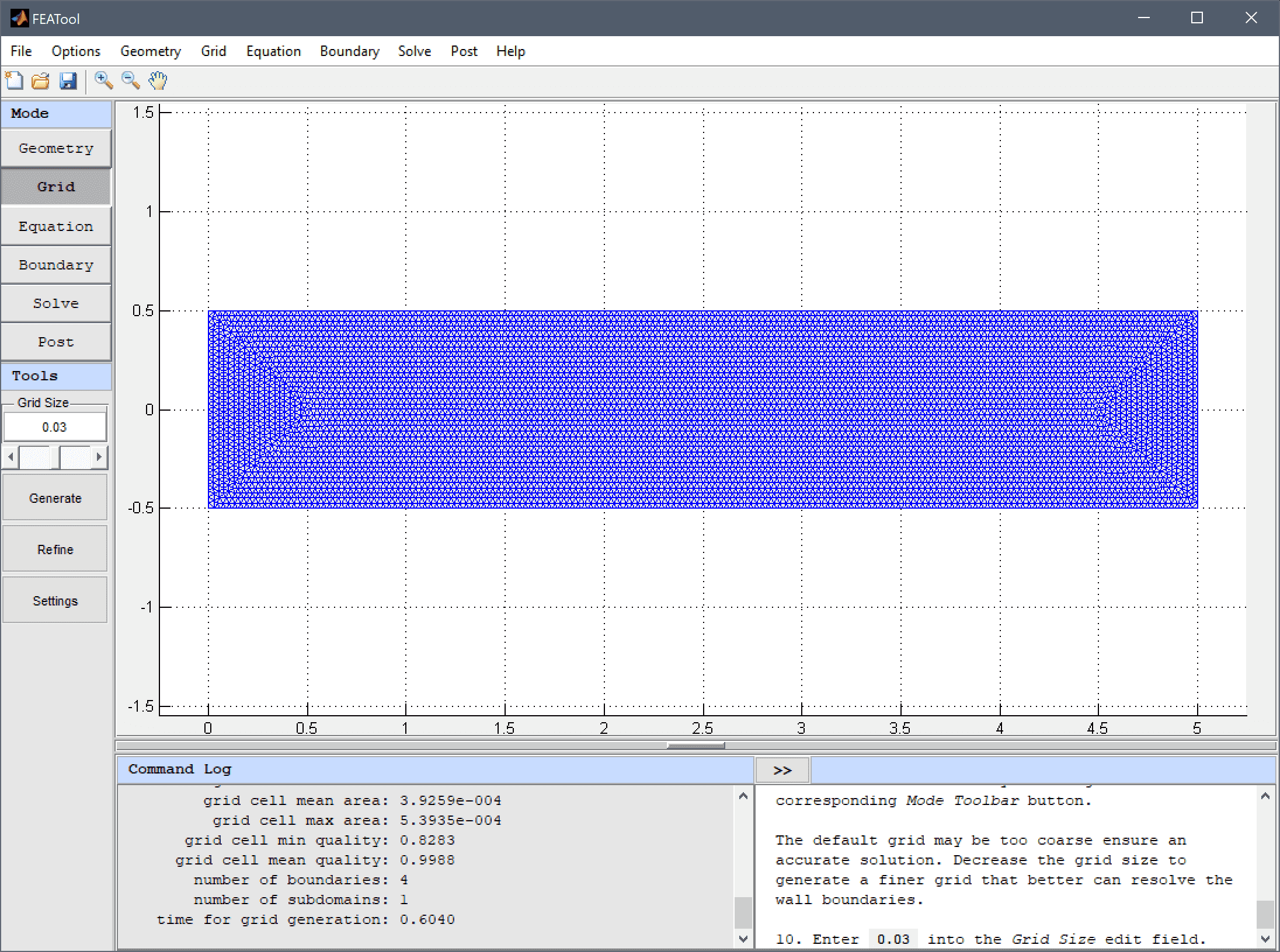
The default grid may be too coarse to ensure an accurate solution. Decrease the grid size to generate a finer grid that better can resolve the wall boundaries which are expected to feature sharp flow gradients.

1. Enter 0.03 into the Grid Size edit field and press the Generate button to call the automatic grid generation algorithm.

   

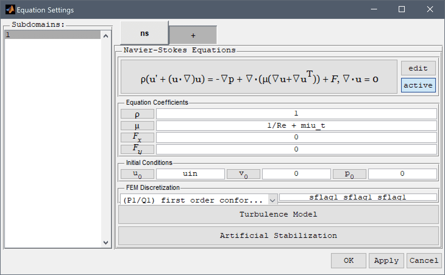
2. Equation and material coefficients are specified in Equation/Subdomain mode. In the Equation Settings dialog box that automatically opens when switching to Equation mode, enter 1 for the fluid Density, 1/Re for the Viscosity, and uin for the initial velocity in the x-direction u₀.

   

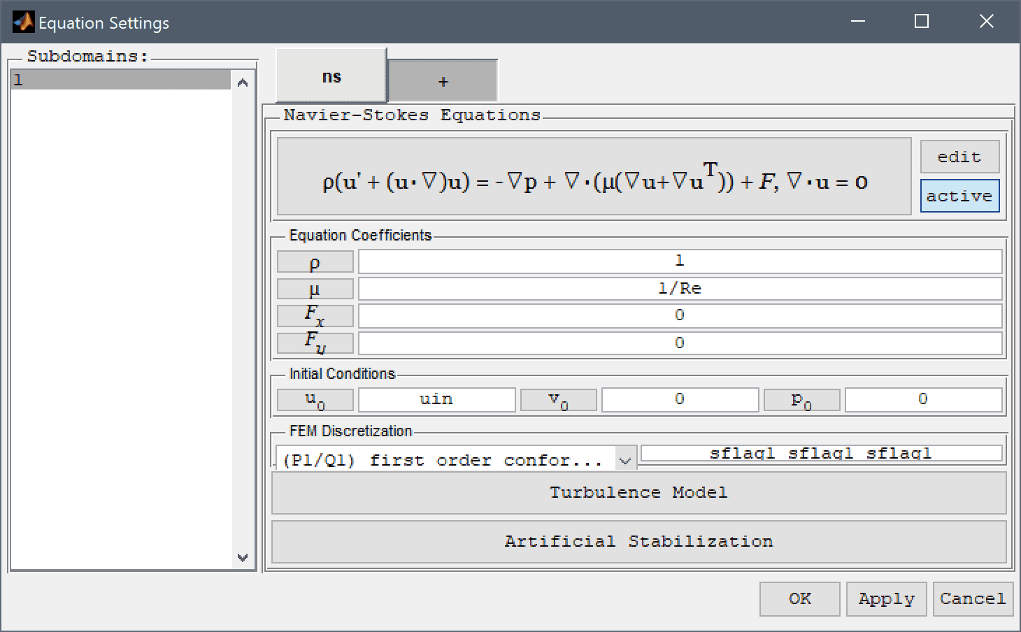
Note that FEATool works with any unit system, and in this model non-dimensionalized units are used. It is up to the user to use consistent units for geometry dimensions, material, equation, and boundary coefficients.

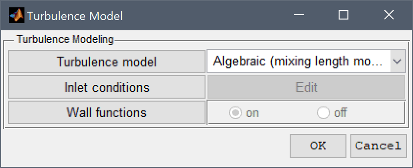
1. Press the Turbulence Model button and select the Algebraic (mixing length model). The algebraic mixing length model is available with the built-in solvers while the more advanced k-epsilon and omega turbulence models requires using the external OpenFOAM CFD solver.

   
2. Press OK to finish the equation and subdomain settings specification.

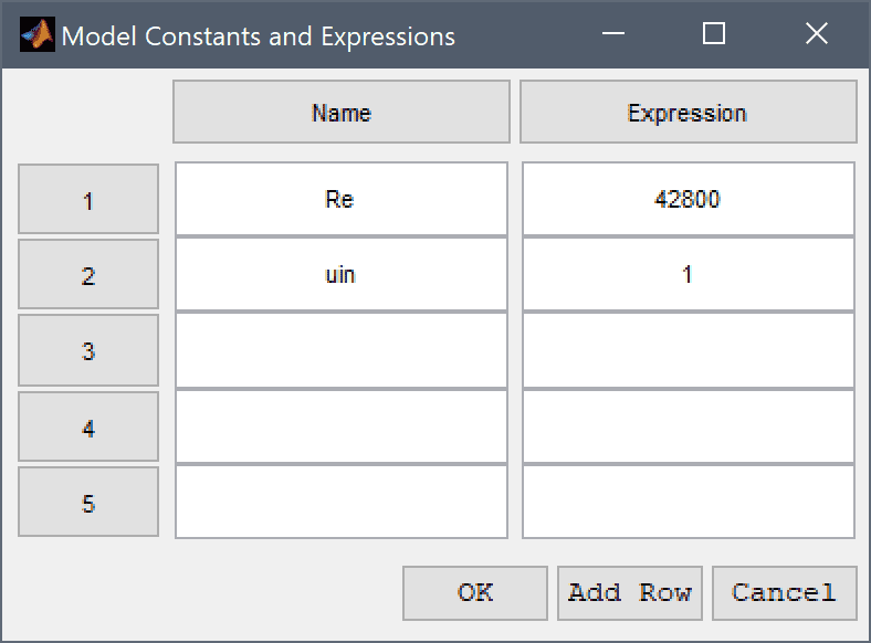
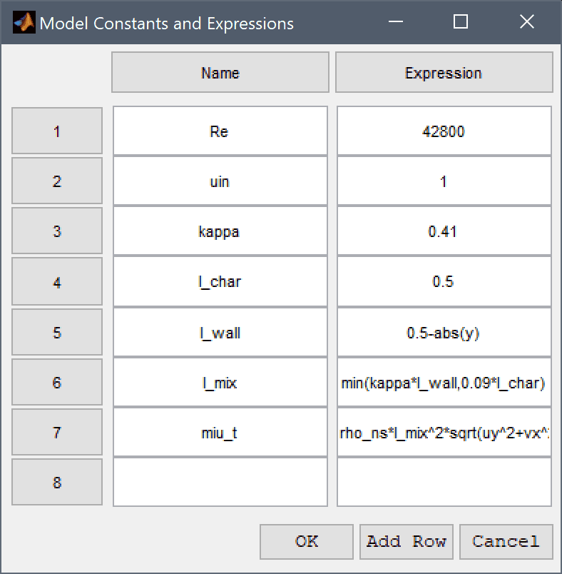
A convenient way to define and store coefficients, variables, and expressions is to use the Model Constants and Expressions functionality. The defined expressions can then be used in point, equation, boundary coefficients, as well as postprocessing expressions, and can easily be changed and updated in a single place.

1. Enter the expressions for the Reynolds number, Re = 42800 which reciprocal is used to define the viscosity, and inlet velocity, uin = 1 used in both the initial and boundary conditions.

   

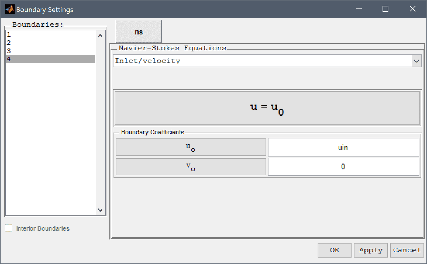
Boundary conditions are defined in Boundary mode and describes how the model interacts with the external environment. Switch to Boundary mode by clicking on the corresponding button.

First select (no-slip) walls for the top and bottom boundaries.

1. Select 1 and 3 in the Boundaries list box.
2. Select Wall/no-slip from the Navier-Stokes Equations drop-down menu.

The fluid flows from left to right, so select an outflow condition for the right boundary.

1. Select 2 in the Boundaries list box.
2. Select Neutral outflow/stress boundary from the Navier-Stokes Equations drop-down menu.

Finally, set the left boundary as an inflow with x-velocity uin.

1. Select 4 in the Boundaries list box.
2. Select Inlet/velocity from the Navier-Stokes Equations drop-down menu.

3. Enter uin into the Velocity in x-direction edit field.

   
4. Press OK to finish the boundary condition specification.
5. Now that the problem is fully specified, press the Solve Mode Toolbar button to switch to solve mode.

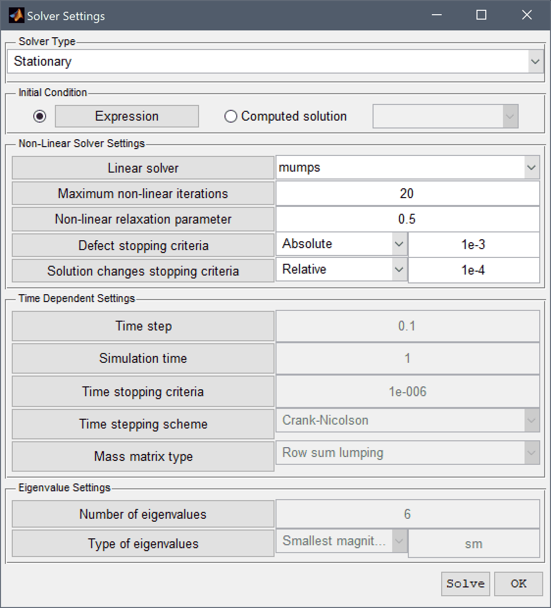
As turbulent flow problems are very non-linear, decrease the non-linear relaxation and tolerances to in the Solver Settings dialog box to help with convergence.

1. Press the Settings Toolbar button.
2. Enter 0.5 into the Non-linear relaxation parameter (ratio of new to old solution to use) edit field.
3. Enter 1e-3 into the Non-linear stopping criteria for solution defects edit field.

4. Enter 1e-4 into the Non-linear stopping criteria for solution differences (changes) between iterations edit field.

   
5. Press OK to apply the selected solver settings.
6. Press the = Tool button to call the solver with the updated solver settings.

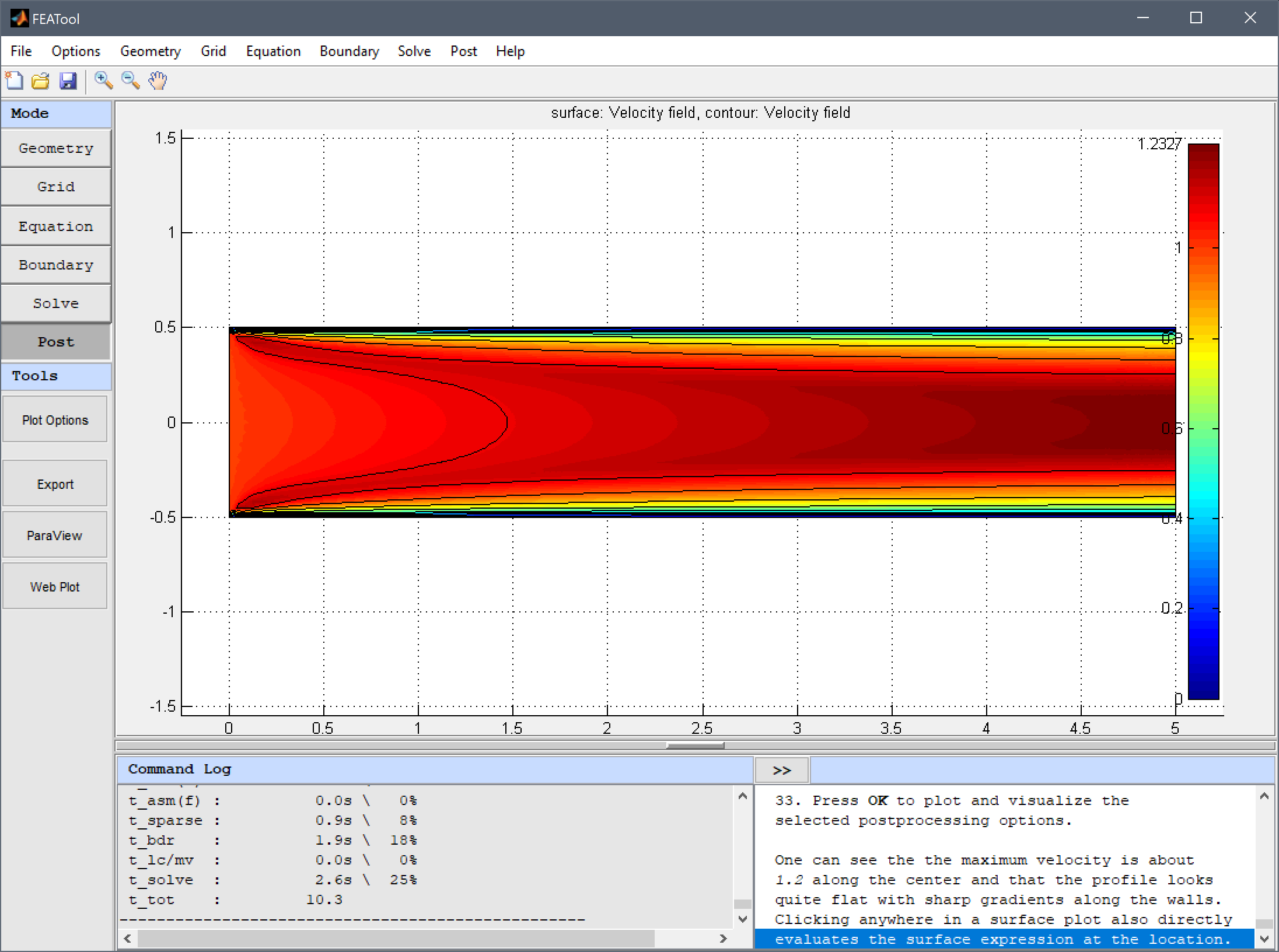
After the problem has been solved FEATool will automatically switch to postprocessing mode and here display the magnitude of the computed velocity field.

1. Press the Plot Options Toolbar button.

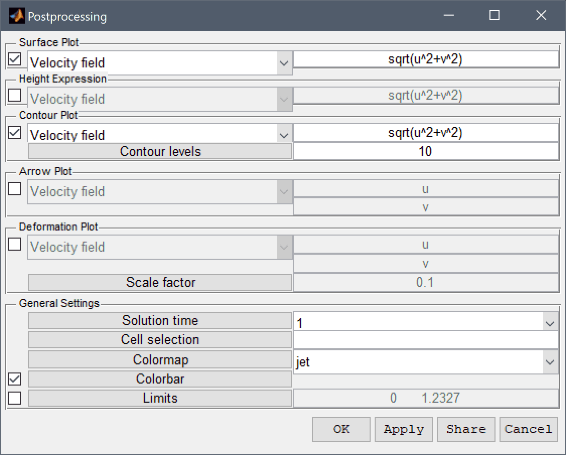
2. Select the Contour Plot check box.

   
3. Press OK to plot and visualize the selected postprocessing options.

One can see that the maximum velocity is about 1.2 along the center and that the profile looks quite flat with sharp gradients along the walls. Clicking anywhere in a surface plot also directly evaluates the surface expression at the location.

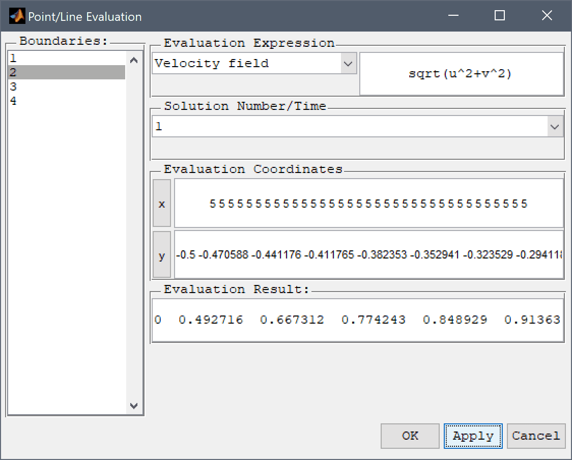
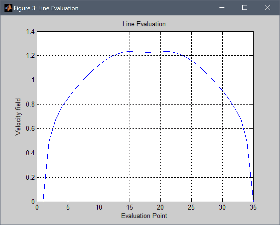
The Point/Line Evaluation menu option can be used to plot a cross section which can show the shape of the turbulent velocity profile more clearly.

1. Select Point/Line Evaluation... from the Post menu.

2. Select 2 in the Boundaries list box.

   
3. Press OK to finish and close the dialog box.

The resulting turbulent velocity profile agrees quite well with the experimental results of Laufer, J. (1950).

1. To implement a custom turbulence model, first go back to Equation mode and turn of the built-in algebraic turbulence model.
2. Press the Turbulence Model button.
3. Select Laminar (no turbulence model) from the Turbulence model drop-down menu.
4. Press OK to plot the selected expression in a new figure and close the dialog box.

A custom expression for the turbulence viscosity will be defined and incorporated so that the total viscosity equals the molecular plus the turbulent viscosity.

1. Enter 1/Re + miu_t into the Viscosity edit field.

   
2. Press OK to finish the equation and subdomain settings specification.

The expression for the custom mixing length model is here defined as rho*l_mix^2*sqrt(uy^2+vx^2) where the mixing length l_mix is defined as min(kappa*l_wall,0.09*l_char). The von Karman constant kappa is 0.41, l_wall is the minimum distance from the walls, and l_char the characteristic length is taken as the maximum of l_wall.

1. Add the following expressions for the turbulence model in the Model Constants and Expressions dialog box. Note that we are not restricted to constants but can freely use mathematical expressions involving other variables.

Name	Expression
kappa	0.41
l_char	0.5
l_wall	0.5-abs(y)
l_mix	min(kappa*l_wall,0.09*l_char)
miu_t	rho_ns*l_mix^2*sqrt(uy^2+vx^2)

1. Switch back to Solve mode again and press the = Tool button to solve the problem with the new custom modeling expression.

The new solution with a custom expression for the turbulence model is very similar to both the built-in model and reference.

The turbulent channel flow fluid dynamics model has now been completed and can be saved as a binary (.fea) model file, or exported as a programmable MATLAB m-script text file (available as the example ex_navierstokes17 script file), or GUI script (.fes) file.