Fluid flows with swirl effects can occur in rotationally symmetric geometries with non-zero azimuthal or angular velocity. In this case one must generally solve the full 3D Navier-Stokes equations. However, if the azimuthal variations can be neglected, simulations can be limited to axisymmetric 2D domains and thus save significant amounts of computational time.

This example models axisymmetric flow between two concentric cylinders where the inner cylinder is rotating. This leads to swirl effects and so called Taylor-Couette flow with periodic and in-plane vortices.

Tutorial

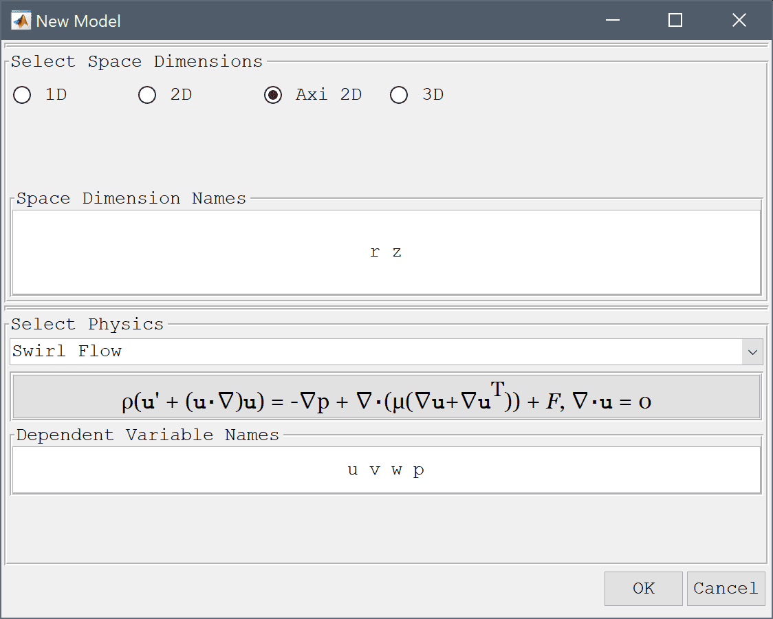
This model is available as an automated tutorial by selecting Model Examples and Tutorials... > Fluid Dynamics > Taylor-Couette Swirling Flow from the File menu. Or alternatively, follow the step-by-step instructions below. Note that the CFDTool interface differ slightly from the FEATool Multiphysics instructions described in the following.

To start a new model click the New Model toolbar button, or select New Model... from the File menu.
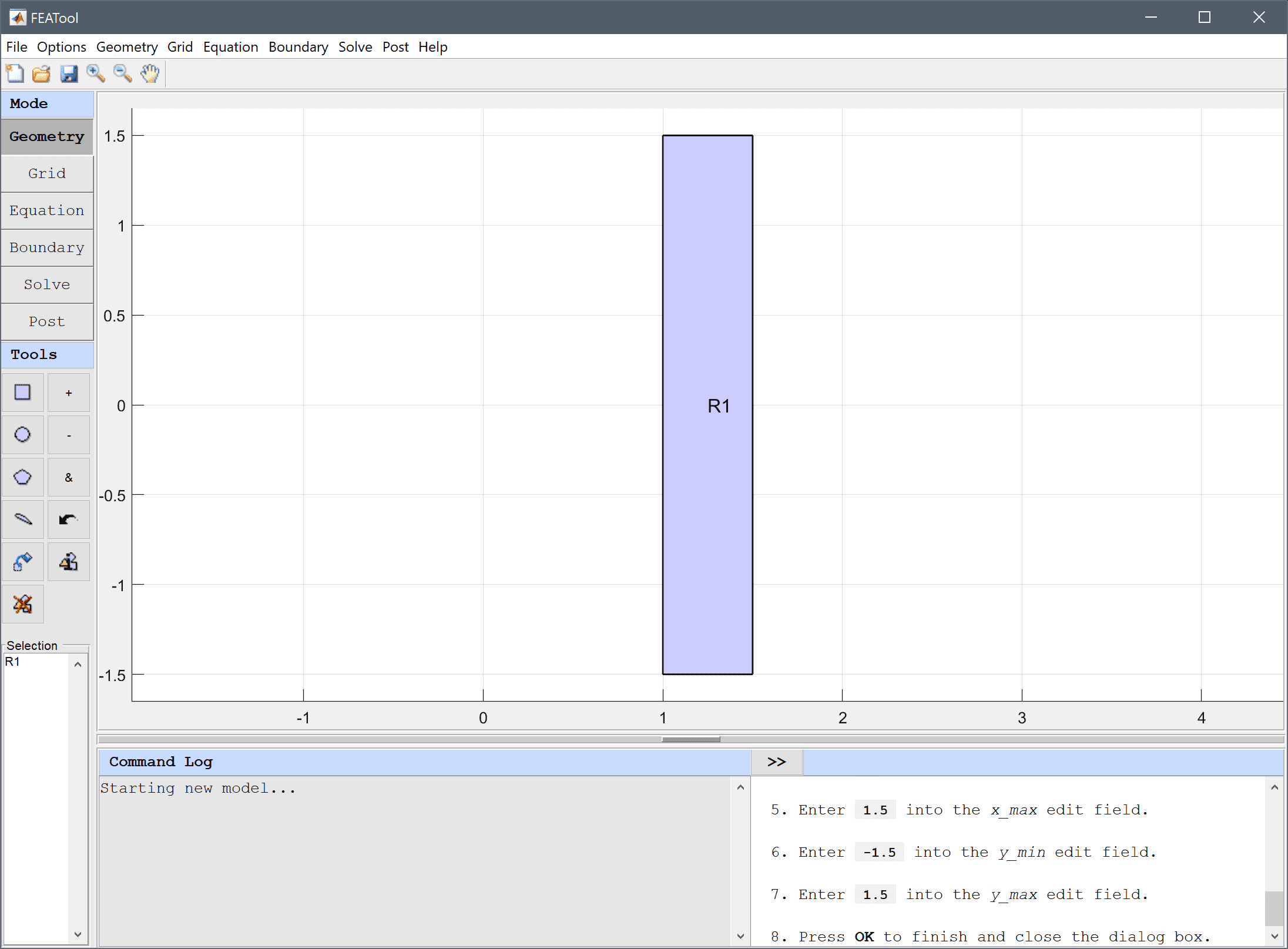
Click on the Axisymmetry Space Dimension selection button in the New Model dialog box, and select Swirl Flow from the Select Physics drop-down list. Leave the space dimension and dependent variable names to their default values. Finish the physics selection and close the dialog box by clicking on the OK button. (Note that for CFDTool the physics selection is done in the Equation settings dialog box.)

The geometry of consists of a rectangular cross section of the cylinder (axisymmetric geometries must be defined in the r>0 positive half plane).

Select Rectangle from the Geometry menu.
Enter 1 into the x_min edit field.
Enter 1.5 into the x_max edit field.
Enter -1.5 into the y_min edit field.
Enter 1.5 into the y_max edit field.
Press OK to finish and close the dialog box.
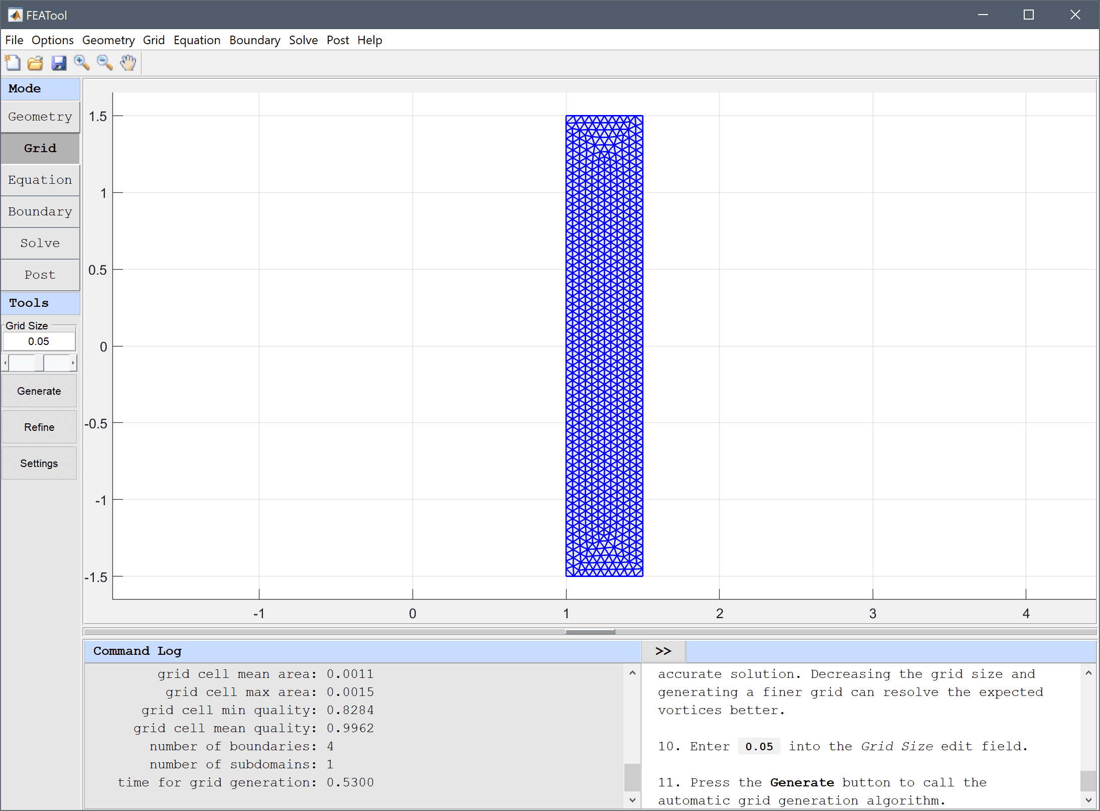
Switch to Grid mode by clicking on the corresponding Mode Toolbar button.

The default grid may be too coarse to ensure an accurate solution. Decreasing the grid size and generating a finer grid can resolve the expected vortices better.

Press the Settings Toolbar button.
Select Gridgen2D from the Grid generation algorithm drop-down menu.
Enter 0.05 into the Subdomain Grid Size edit field.
Press OK to finish and close the dialog box.
Press the Generate button to call the automatic grid generation algorithm.

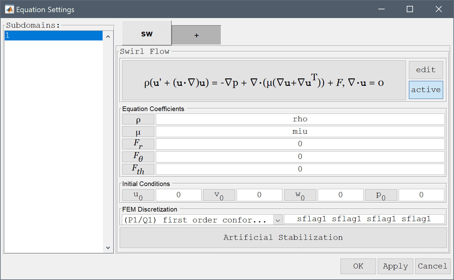
Switch to Equation mode by clicking on the corresponding Mode Toolbar button.
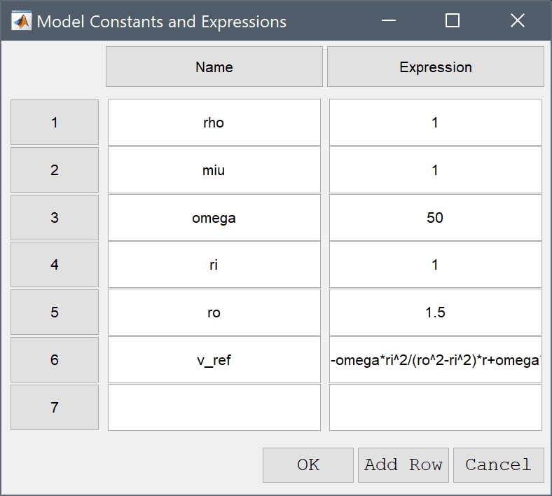
Equation and material coefficients are specified in Equation/Subdomain mode. In the Equation Settings dialog box enter rho for the density and miu for the viscosity. Then press OK to finish with specifications the equation coefficients. (Note that the Equation Settings dialog box may look different for CFDTool.)

The Model Constants and Expressions functionality can be used to define and store convenient expressions which then are available in the point, equation, boundary coefficients, and as postprocessing expressions. Here it is used to define the fluid coefficients, angular velocity, inner and outer radius, and reference solution.

Press the Constants Toolbar button, or select the corresponding entry from the Equation menu, and enter the following variables in the Model Constants and Expressions dialog box. Press Enter after the last expression or use the Add Row button to expand the expression list.

Name	Expression
rho	1
miu	1
omega	50
ri	1
ro	1.5
v_ref	-omegari^2/(ro^2-ri^2)r+omega*ro^2/(ro^2-ri^2)/r

Note that FEATool can work with any unit system, and it is up to the user to use consistent units for geometry dimensions, material, equation, and boundary coefficients.

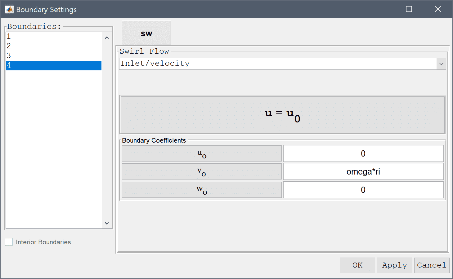
Switch to boundary condition specification mode by clicking on Boundary the Mode Toolbar button.

Boundary conditions are defined in Boundary Mode and describes how the model interacts with the external environment.

In the Boundary Settings dialog box, first choose boundaries 1-3 in the left hand side Boundaries list box and select the Wall/no-slip boundary condition from the drop-down menu.
Then select the inner rotating boundary (number 4) in the left hand side Boundaries list box and select the Inlet/velocity boundary condition. Enter omega*ri in the edit field to specify the velocity v₀ in the tangential-direction.
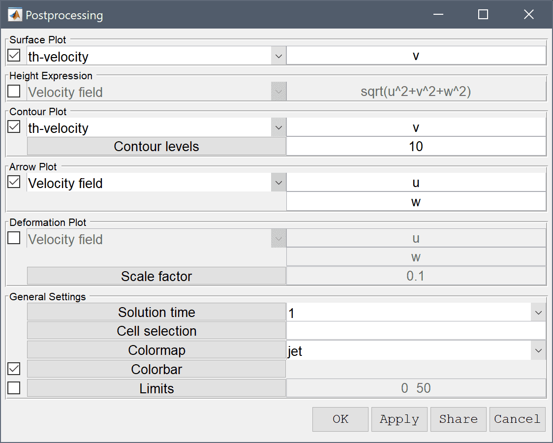
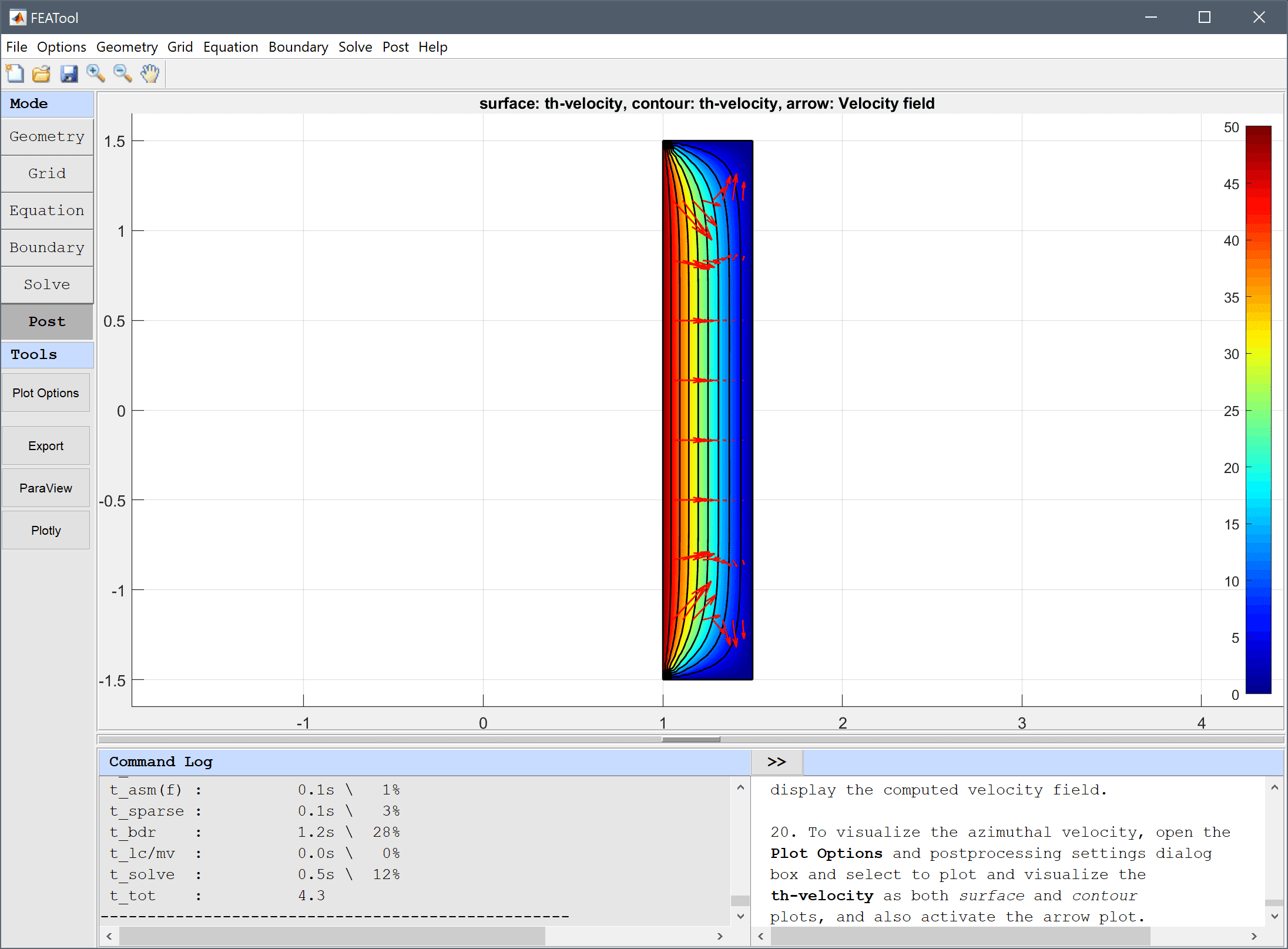
Press OK to finish the boundary condition specification.
Now that the problem is fully specified, press the Solve Mode Toolbar button to switch to solve mode. Then press the = Tool button to call the solver with the default solver settings.

After the problem has been solved FEATool will automatically switch to postprocessing mode and display the computed velocity field.

To visualize the azimuthal velocity, open the Plot Options and postprocessing settings dialog box and select to plot and visualize the th-velocity as both surface and contour plots, and also activate the arrow plot.

One can study a section of the velocity profile by using the Point/Line Evaluation... feature from the Post menu. By entering a series of evaluation coordinates, both the evaluated expression and a corresponding cross section plot can be generated.

Create line plots of both the computed azimuthal velocity and the analytic expression previously defined as v_ref.

Select Point/Line Evaluation... from the Post menu.
Enter 1:0.01:1.5 into the Evaluation coordinates in r-direction edit field.
Enter 0 into the Evaluation coordinates in z-direction edit field.
Select th-velocity from the Evaluation Expression drop-down menu.
Press the Apply button.
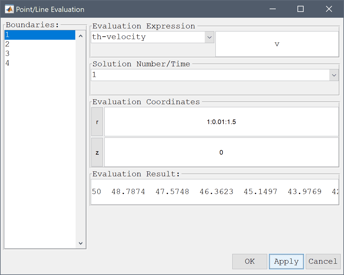
Enter v_ref into the edit field.
Press OK to finish and close the dialog box.

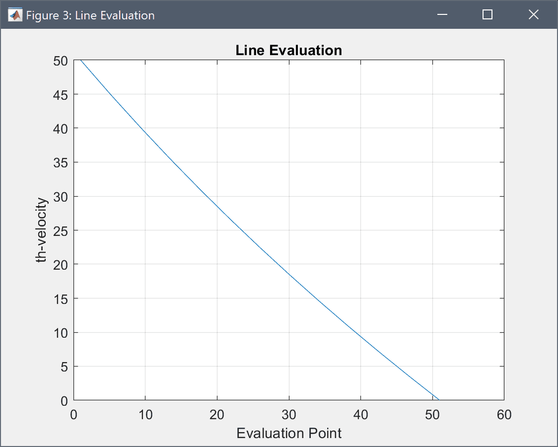
From comparing the curves it should be clear that the simulation produces the expected results.

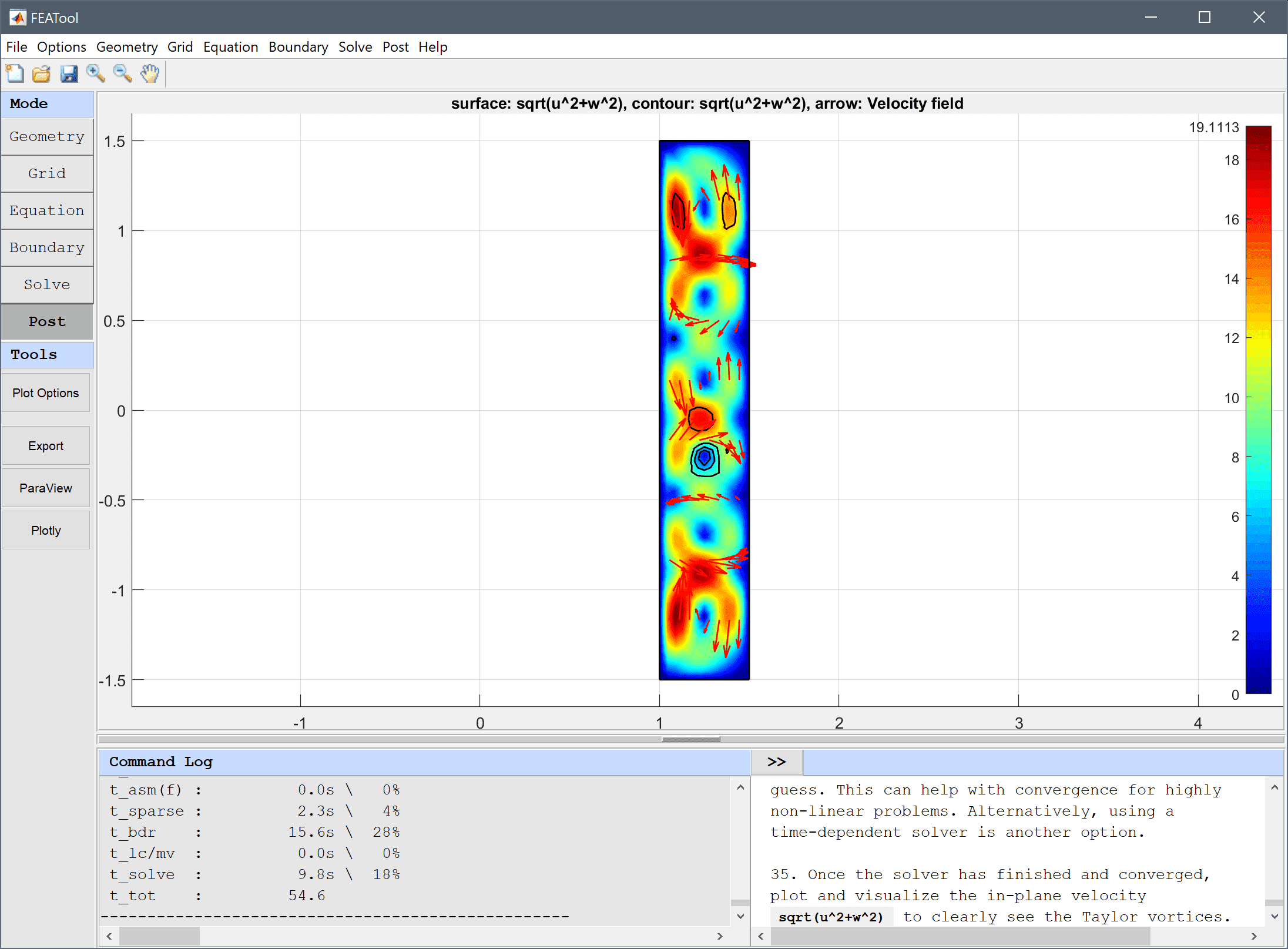
If the rotational velocity is increased beyond the critical Taylor number periodic in-plane vortices will appear.

Open the Model Constants and Expressions... dialog box again and increase omega to 175.

Return to Solve mode again, open the Solver Settings dialog box.
Enter 1e-4 into the Non-linear stopping criteria for solution defects edit field.
Enter 275 into the Maximum number of non-linear iterations edit field.
Press OK to apply the selected solver settings.
This time use the Restart button to start the solver with the previous solution as initial guess. This can help with convergence for highly non-linear problems. Alternatively, using a time-dependent solver is another option.
Once the solver has finished and converged, plot and visualize the in-plane velocity sqrt(u^2+w^2) to clearly see the Taylor vortices.

The Taylor-Couette swirling flow fluid dynamics model has now been completed and can be saved as a binary (.fea) model file, or exported as a programmable MATLAB m-script text file, or GUI script (.fes) file.

Swirl Flow Using The CLI

With FEATool one can also conveniently program and script the models on the MATLAB command line interfaces (CLI). The following example sets up a model for flow between two cylinders where the inner one is rotating and the outer is stationary. The first step is to define the model parameters, geometry, and grid

% Problem definition.
rho   = 1.0;   % Density.
miu   = 1.0;   % Molecular viscosity.
omega = 5.0;   % Angular velocity.
ri    = 0.5;   % Inner radius.
ro    = 1.5;   % Outer radius.
h     = 3.0;   % Height of cylinder.

% Geometry and grid generation.
fea.sdim = {'r' 'z'};
fea.geom.objects = { gobj_rectangle(ri,ro,-h/2,h/2) };
fea.grid = gridgen( fea, 'hmax', (ro-ri)/6 );

Next the, governing equations are defined, here directly without using any predefined physics modes

% Equation definition.
fea.dvar = { 'u', 'v', 'w', 'p' };
fea.sfun = [ repmat( {'sflag2'}, 1, 3 ) {'sflag1'} ];
c_eqn    = { 'r*rho*u'' - r*miu*(2*ur_r + uz_z  +   wr_z) + r*rho*(u*ur_t + w*uz_t) + r*p_r     = - 2*miu/r*u_t + p_t + rho*v*v_t';
             'r*rho*v'' - r*miu*(  vr_r + vz_z) + miu*v_r + r*rho*(u*vr_t + w*vz_t) + rho*u*v_t = miu*(v_r - 1/r*v_t)';
             'r*rho*w'' - r*miu*(  wr_r + uz_r  + 2*wz_z) + r*rho*(u*wr_t + w*wz_t) + r*p_z     = 0';
             'r*ur_t + r*wz_t + u_t = 0' };
fea.eqn = parseeqn( c_eqn, fea.dvar, fea.sdim );

fea.coef = { 'rho', rho ;
             'miu', miu };

For boundary conditions the inner wall is given a rotational velocity, while the outer is prescribed a no-slip wall, and the top and bottom zero normal flows

% Boundary conditions.
fea.bdr.d = { []  0 []  0 ;
              []  0 [] omega*ri ;
               0  0  0 [] ;
              [] [] [] [] };
fea.bdr.n = cell(size(fea.bdr.d));

The incompressible Navier-Stokes equations typically requires the pressure to be defined and fixed in at least one point. This is usually done with an outflow boundary, but since here there are no in- or out-flows, the pressure is simply fixed by setting the value of the top outer corner to zero

% Fix pressure at p([r,z]=[ro,h/2]) = 0.
[~,ix_p] = min( sqrt( (fea.grid.p(1,:)-ro).^2 + (fea.grid.p(2,:)-h/2).^2) );
fea.pnt = struct( 'type',  'constr', 'index', ix_p, 'dvar', 'p', 'expr', '0' );

To improve convergence, and compute a stationary solution faster, an analytic Newton Jacobian is defined (the non-linear Newton solver is activated when the jac solver argument is provided, otherwise standard fix-point iterations are used)

% Define analytical Newton Jacobian bilinear form.
jac.coef  = { 'r*rho*ur'       'rho*v' 'r*rho*uz' [] ;
              'r*rho*vr+rho*v' []      'r*rho*vz' [] ;
              'r*rho*wr'       []      'r*rho*wz' [] ;
              []               []      []         [] };
jac.form = cell(size(jac.coef));
[jac.form{~cellfun(@isempty,jac.coef)}] = deal([1;1]);

The complete problem can now be parsed and solved

% Parse and solve problem.
fea = parseprob( fea );
fea.sol.u = solvestat( fea, 'jac', jac );

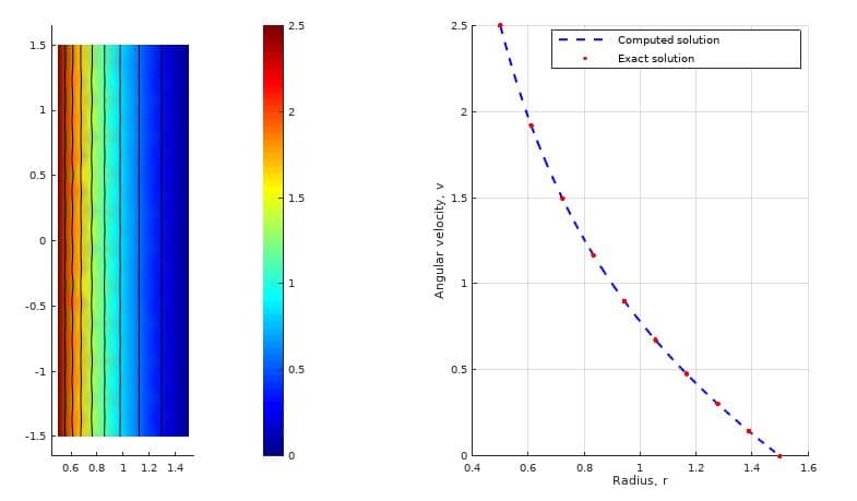
To verify the accuracy of the computed solution a comparison with an analytic solution (valid for small rotational velocities) is made

% Exact (analytical) solution.
a = - omega*ri^2 / (ro^2-ri^2);
b =   omega*ri^2*ro^2 / (ro^2-ri^2);
v_th_ex = @(r,a,b) a.*r + b./r;

% Postprocessing.
subplot(1,2,1)
postplot( fea, 'surfexpr', 'sqrt(u^2+v^2+w^2)', 'isoexpr', 'v' )

subplot(1,2,2)
hold on
grid on
r = linspace( ri, ro, 100 );
v_th = evalexpr( 'v', [r;zeros(1,length(r))], fea );
plot( r, v_th, 'b--' )
r = linspace( ri, ro, 10 );
plot( r, v_th_ex(r,a,b), 'r.' )
legend( 'Computed solution', 'Exact solution')
xlabel( 'Radius, r')
ylabel( 'Angular velocity, v')

From the figure below it is clear that very good agreement with the analytical solution has been achieved.

A time-dependent Taylor-Couette flow script model is available from the FEATool models and examples directory as the ex_swirl_flow3 model m-script file (note that periodic boundary conditions are implemented with an external solve_hook function.