|
|
FEATool Multiphysics
v1.18.0
Finite Element Analysis Toolbox
|
|
|
FEATool Multiphysics
v1.18.0
Finite Element Analysis Toolbox
|
This is an example of modeling anisotropic heat conduction in an orthotropic material where a heated solid bar suddenly is cooled by submerging it in a cool fluid. The material features different thermal conductivities in the x and y-directions which is accounted for by modifying the diffusion term in the heat transfer equation. Instead of solving the usual isotropic case
\[ \rho C_p\frac{\partial T}{\partial t} - k(\frac{\partial^2 T}{\partial x^2} + \frac{\partial^2 T}{\partial x^2}) = 0 \]
we will instead solve the following
\[ \rho C_p\frac{\partial T}{\partial t} - (k_x\frac{\partial^2 T}{\partial y^2} + k_y\frac{\partial^2 T}{\partial y^2}) = 0 \]
where \(k_x = 34.6147\) and \(k_y = 6.23687\ W/mK\) are the thermal conductivities in the different directions. Fully anisotropic cases can technically also be handled by introducting off-diagonal \(k_{x_i,x_j}\frac{\partial^2 T}{\partial x_i \partial x_j}\) diffusion terms.
The following material and simulation parameters are given; initial temperature \(T_0 = 260\ °C\), density \(\rho = 6407.4 \ kg/m^3\), heat capacity \(C_p = 37.688\ J/kgK\). Due to symmetry we only need to model a quarter domain of a 2D cross-section with dimensions 5.08 by 2.54 cm. Conductive heat flux boundary conditions are used on the external boundaries with a convection coefficient \(h = 1361.7\ W/m^2K\) and surrounding temperature \(T_{inf} = 37.7778\ °C\). The cooling process is simulated for 3 seconds after which the temperature is measured in the center core and corners, and compared to the reference values [1].
This section describes how to set up and solve the orthotropic heat conduction example with the FEATool graphical user interface (GUI).
The model is available as an automated tutorial by selecting Model Examples and Tutorials... > Heat Transfer > Orthotropic Heat Conduction from the File menu. Or alternatively, follow the step-by-step instructions below.
Select the Heat Transfer physics mode from the Select Physics drop-down menu.
Due to symmetry we only need to model a quarter of the domain, a 1 by 2 inch rectangle. Note that as FEATool does not specify a fixed unit system the dimensions are converted to SI units for convenience and to be consistent with the units used in the material parameters.
2*2.54*1e-2 into the xmax edit field.Enter 1*2.54*1e-2 into the ymax edit field.
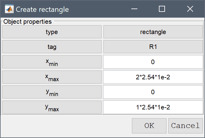
Press OK to finish and close the dialog box.
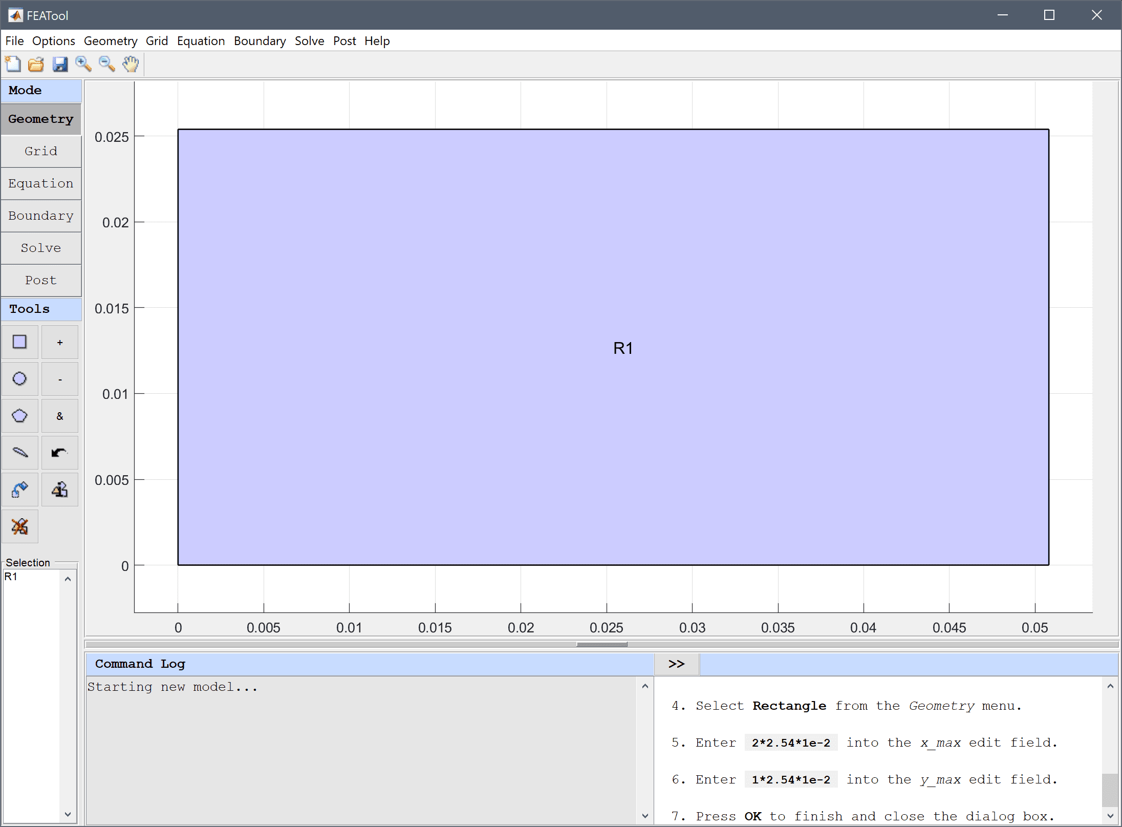
Increase the grid density by pressing the Refine Toolbar button twice.
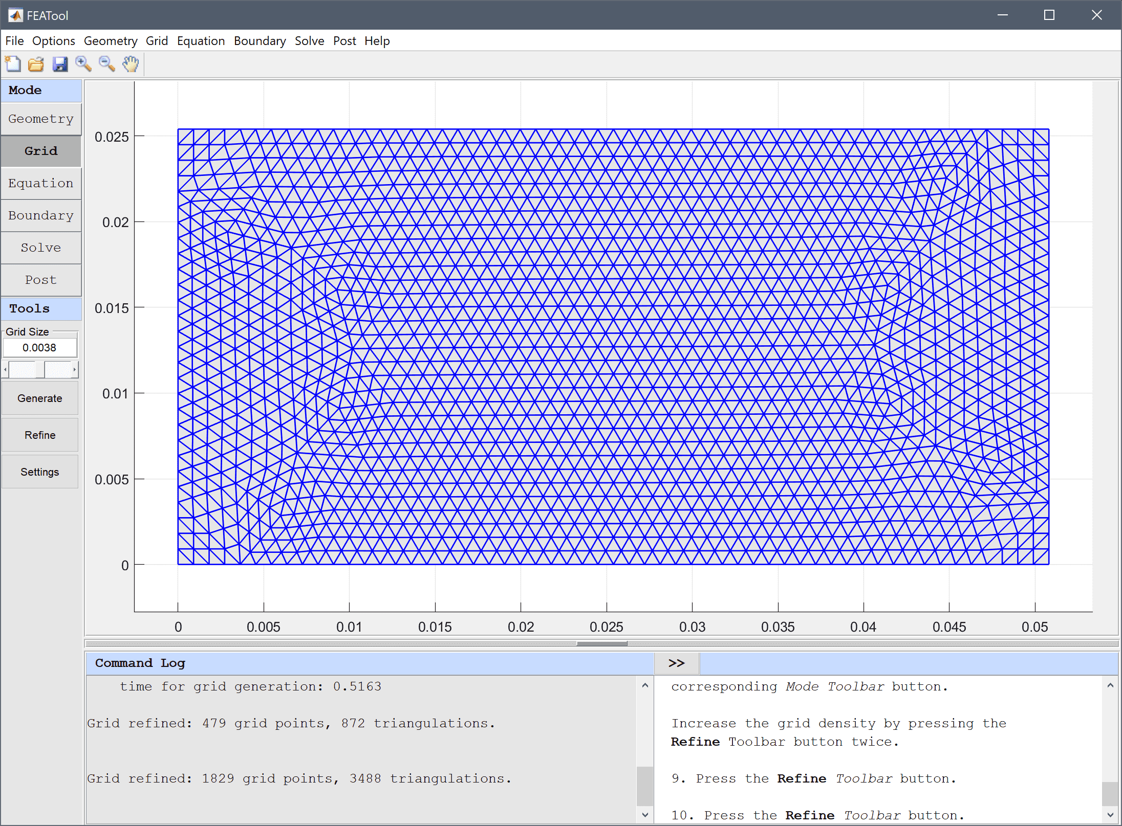
6407.4 into the Density edit field.37.688 into the Heat capacity edit field.Enter 260 into the Initial condition for T edit field.
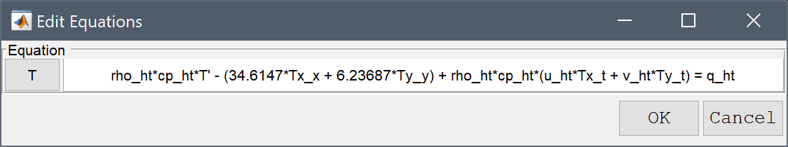
To model the anisotropic diffusion coefficient edit the heat transfer equation and replace the original term k_ht*(Tx_x + Ty_y) with (34.6147*Tx_x + 6.23687*Ty_y).
Enter rho_ht*cp_ht*T' - (34.6147*Tx_x + 6.23687*Ty_y) + rho_ht*cp_ht*(u_ht*Tx_t + v_ht*Ty_t) = q_ht into the Equation for T edit field.
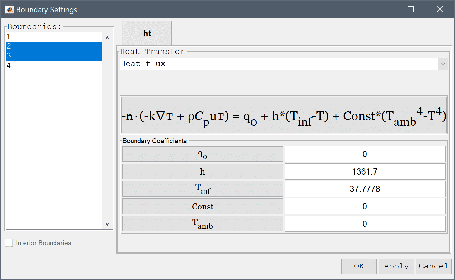
Boundary conditions are defined in Boundary Mode and describes how the model interacts with the external environment. Here the bottom and left sides are symmetry boundaries while the top and right are prescribed convective flux conditions.
1361.7 into the Heat transfer coefficient edit field.Enter 37.7778 into the Bulk temperature edit field.
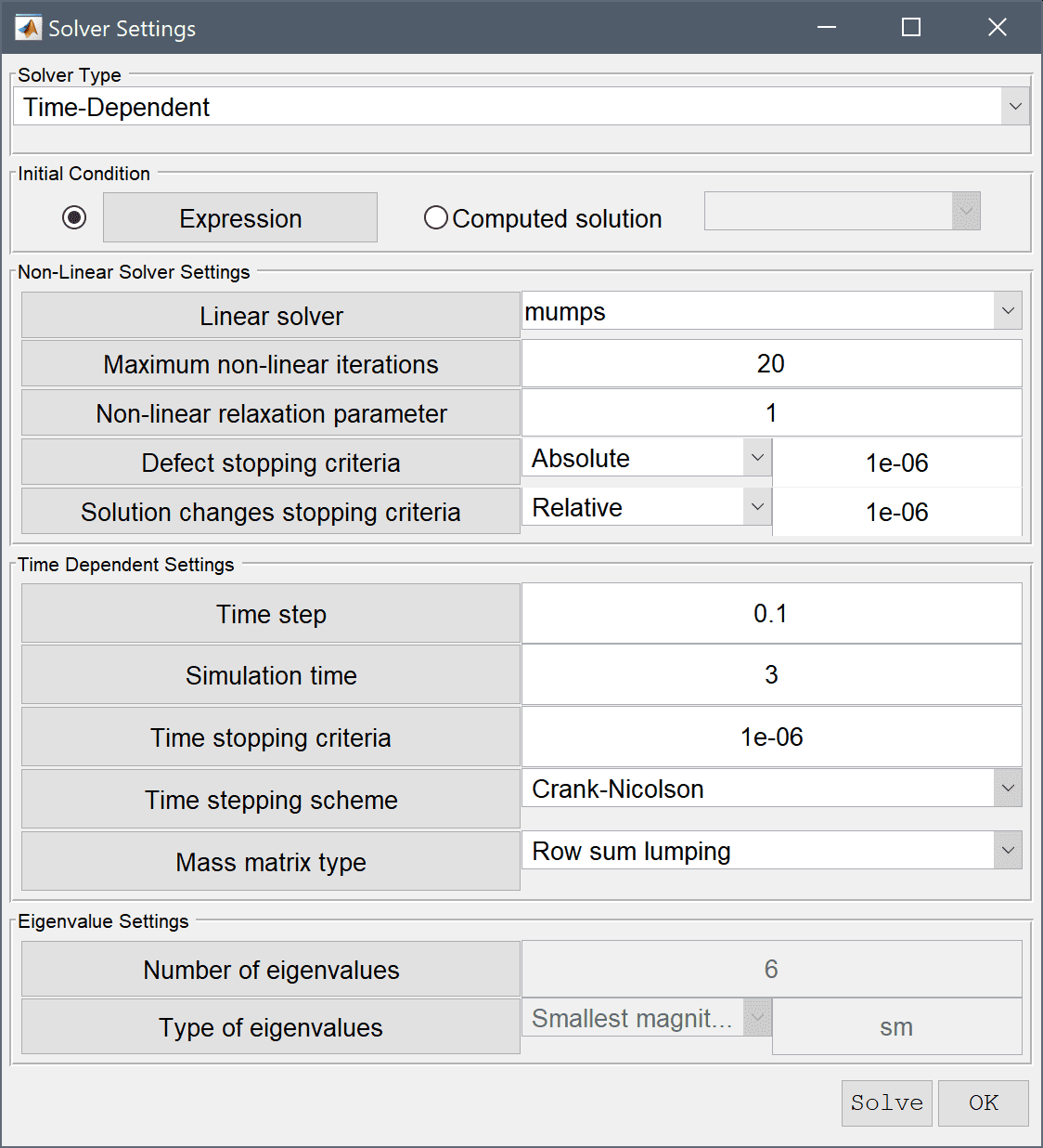
Enter 3 into the Duration of time-dependent simulation (maximum time) edit field.
20 into the Number or specified vector of contour levels to plot edit field.Press OK to plot and visualize the selected postprocessing options.
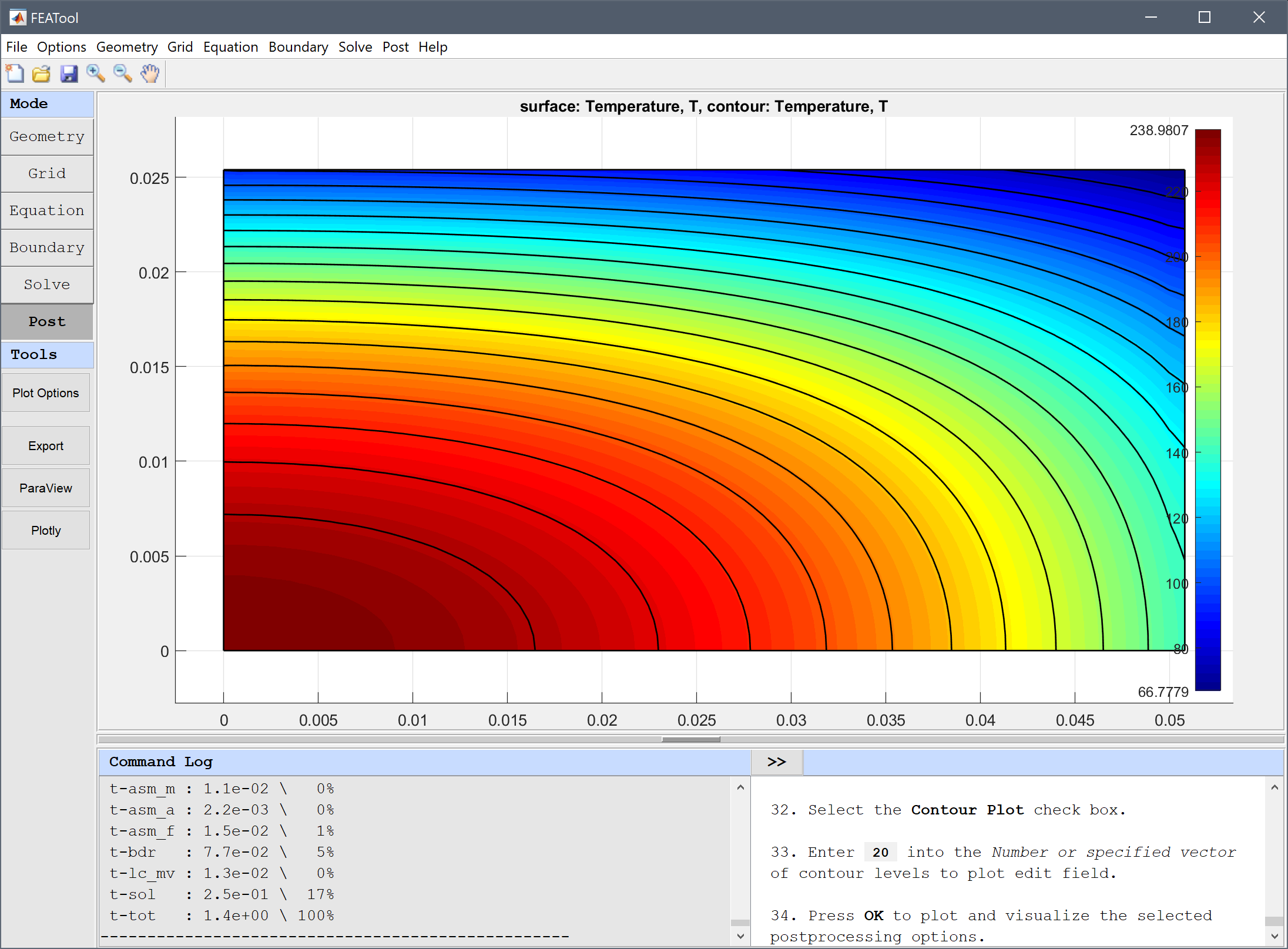
To evaluate the accuracy of the solution the temperature can be evaluated in the points (0,0), (2,1), (2,0), and (0,1) inches and compared with reference temperature values \(T_{ref}\) = 237, 66.1, 137, and 94.4 degrees C respectively.
0 0.0508 0.0508 0 into the Evaluation coordinates in x-direction edit field.0 0.0254 0 0.0254 into the Evaluation coordinates in y-direction edit field.Press the Apply button.
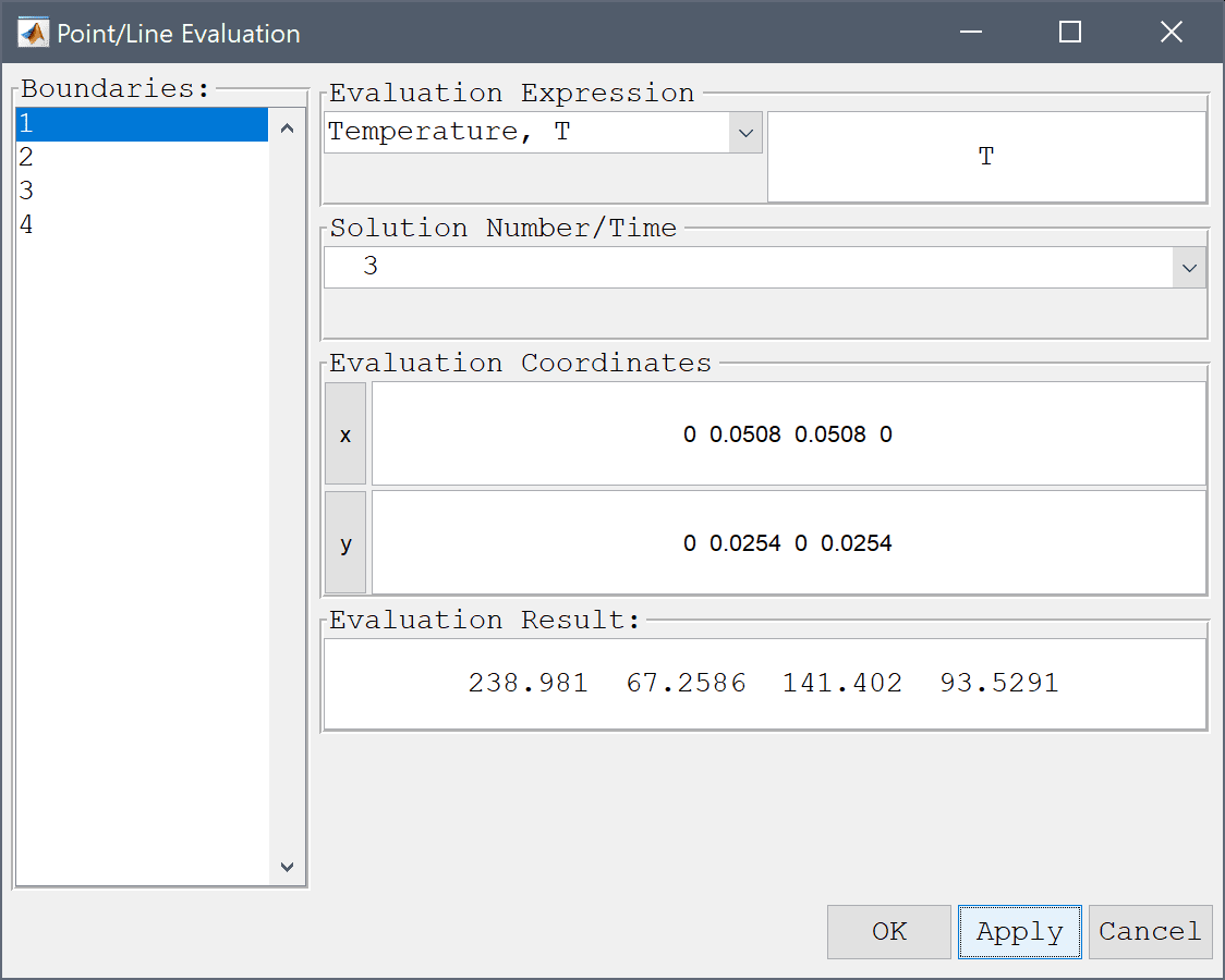
From the Evaluation Result field we can see that the computed temperature in the evaluation points is very close to the reference values.
The orthotropic heat conduction heat transfer model has now been completed and can be saved as a binary (.fea) model file, or exported as a programmable MATLAB m-script text file, or GUI script (.fes) file.
[1] P.J. Schneider, Conduction Heat Transfer, Addison-Wesley, 2nd Ed., Ex. 10-7, pp. 261, 1957.