Thermal Bridge

This is a benchmark test case for modeling the steady-state temperature distribution in a thermal bridge in building construction [1]. The model consists of a 6 mm concrete slab subjected to an outside temperature of 0 degrees and heat loss due to convection. The inside features a 4 cm layer of air enclosed within a 1.5 mm metal frame, which is attached to the slab with an insulating layer. The inside temperature is assumed a constant 20 degrees. The model can both be considered to be planar, and also symmetric at the ends so that only a 2D 0.5 m section needs to be modeled. The heat flux and temperature at various points is compared to given reference values [1].

Tutorial

The following section describes how to set up and solve the thermal bridge validation model with the FEATool graphical user interface (GUI).

This model is available as an automated tutorial by selecting Model Examples and Tutorials... > Heat Transfer > Thermal Bridge from the File menu. Or alternatively, follow the step-by-step instructions below. Note that the CFDTool interface differ slightly from the FEATool Multiphysics instructions described in the following.

1. To start a new model click the New Model toolbar button, or select New Model... from the File menu.

2. Select the Heat Transfer physics mode from the Select Physics drop-down menu. (Note that for CFDTool the physics selection is done in the Equation settings dialog box.)

   
3. Press OK to finish the physics mode selection.

First create a 0.5 by 0.0475 m background rectangle for the domain.

1. Select Rectangle from the Geometry menu.
2. Enter 0 into the x_min edit field.
3. Enter 0.5 into the x_max edit field.
4. Enter 0 into the y_min edit field.
5. Enter 0.0475 into the y_max edit field.
6. Press OK to finish and close the dialog box.

Then create rectangles for the top concrete slab and a smaller one for the insulating layer.

1. Select Rectangle from the Geometry menu.
2. Enter 0 into the x_min edit field.
3. Enter 0.5 into the x_max edit field.
4. Enter 0.0415 into the y_min edit field.
5. Enter 0.0475 into the y_max edit field.
6. Press OK to finish and close the dialog box.
7. Select Rectangle from the Geometry menu.
8. Enter 0 into the x_min edit field.
9. Enter 0.0135 into the x_max edit field.
10. Enter 0.0365 into the y_min edit field.
11. Enter 0.0415 into the y_max edit field.
12. Press OK to finish and close the dialog box.

Finally the polygon tool is used to define the shape of the metal frame.

1. Select Polygon from the Geometry menu and enter the following data into the Point coordinates table.

	x	y
1	0	0
2	0.5	0
3	0.5	0.0015
4	0.0015	0.0015
5	0.0015	0.035
6	0.0135	0.035
7	0.0135	0.0365
8	0	0.0365

1. Press OK to finish and close the dialog box.

   

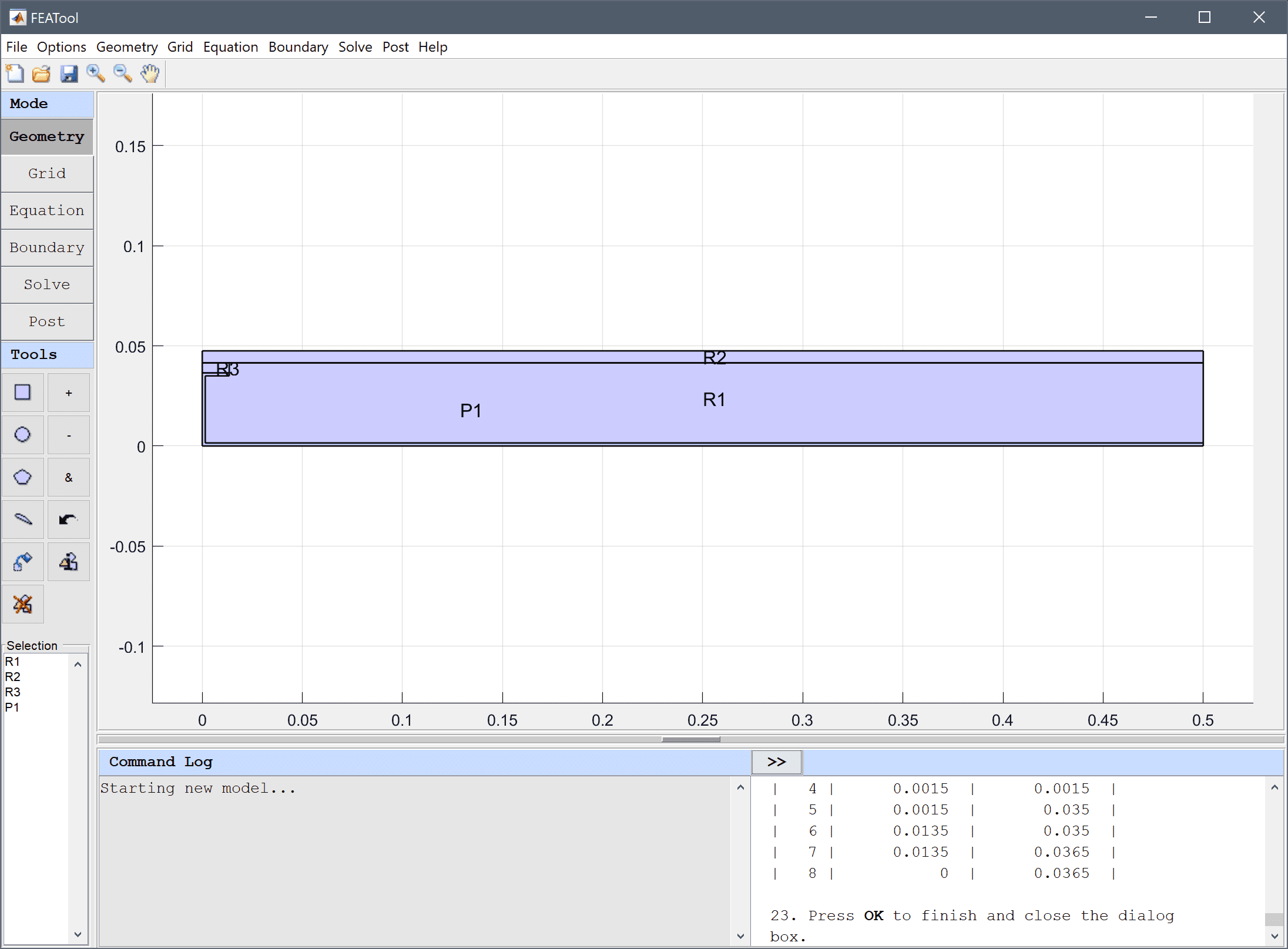
Although some geometry objects overlap, decomposed minimal regions will automatically be generated in the grid generation step.

1. Switch to Grid mode by clicking on the corresponding Mode Toolbar button which automatically generates a default grid for 2D problems.
2. Switch to Equation mode by clicking on the corresponding Mode Toolbar button.

Equation and material coefficients can be specified in Equation/Subdomain mode. In the Equation Settings dialog box that automatically opens select the four subdomains and change the heat coefficient for the thermal conductivity k correspondingly. As the simulation is stationary the density, heat capacity, and other coefficients don't come in to play and can be left to their default values. (Note that the Equation Settings dialog box may look different for CFDTool.)

1. First select the subdomain for the slab, 4 in the Subdomains list box.
2. Enter 1.15 into the Thermal conductivity edit field.
3. Select subdomain 2, the insulation layer, in the Subdomains list box.
4. Enter 0.12 into the Thermal conductivity edit field.
5. Then select subdomain 1 the metal frame.
6. Enter 230 into the Thermal conductivity edit field.
7. Finally select subdomain 3, the domain with air.

8. Enter 0.029 into the Thermal conductivity edit field.

   

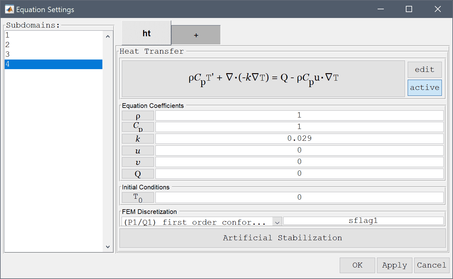
Note that FEATool works with any unit system, and it is up to the user to use consistent units for geometry dimensions, material, equation, and boundary coefficients.

1. Press OK to finish the equation and subdomain settings specification.
2. Switch to Boundary mode by clicking on the corresponding Mode Toolbar button.

In boundary mode, first select the Thermal insulation/symmetry condition for all left and right boundaries.

1. Select 2-6, 8 in the Boundaries list box.
2. Select Thermal insulation/symmetry from the Heat Transfer drop-down menu.

Then select the convective heat flux condition for the top and bottom boundaries.

1. Select 7 in the Boundaries list box.
2. Select Heat flux from the Heat Transfer drop-down menu.
3. Enter 1/0.06 into the Heat transfer coefficient edit field.

4. Enter 0 into the Bulk temperature edit field.

   
5. Select 1 in the Boundaries list box.
6. Select Heat flux from the Heat Transfer drop-down menu.
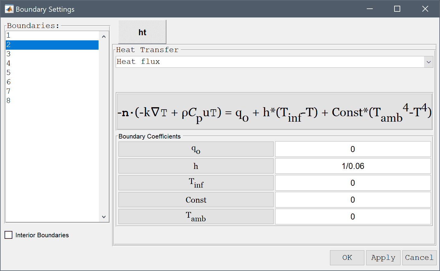
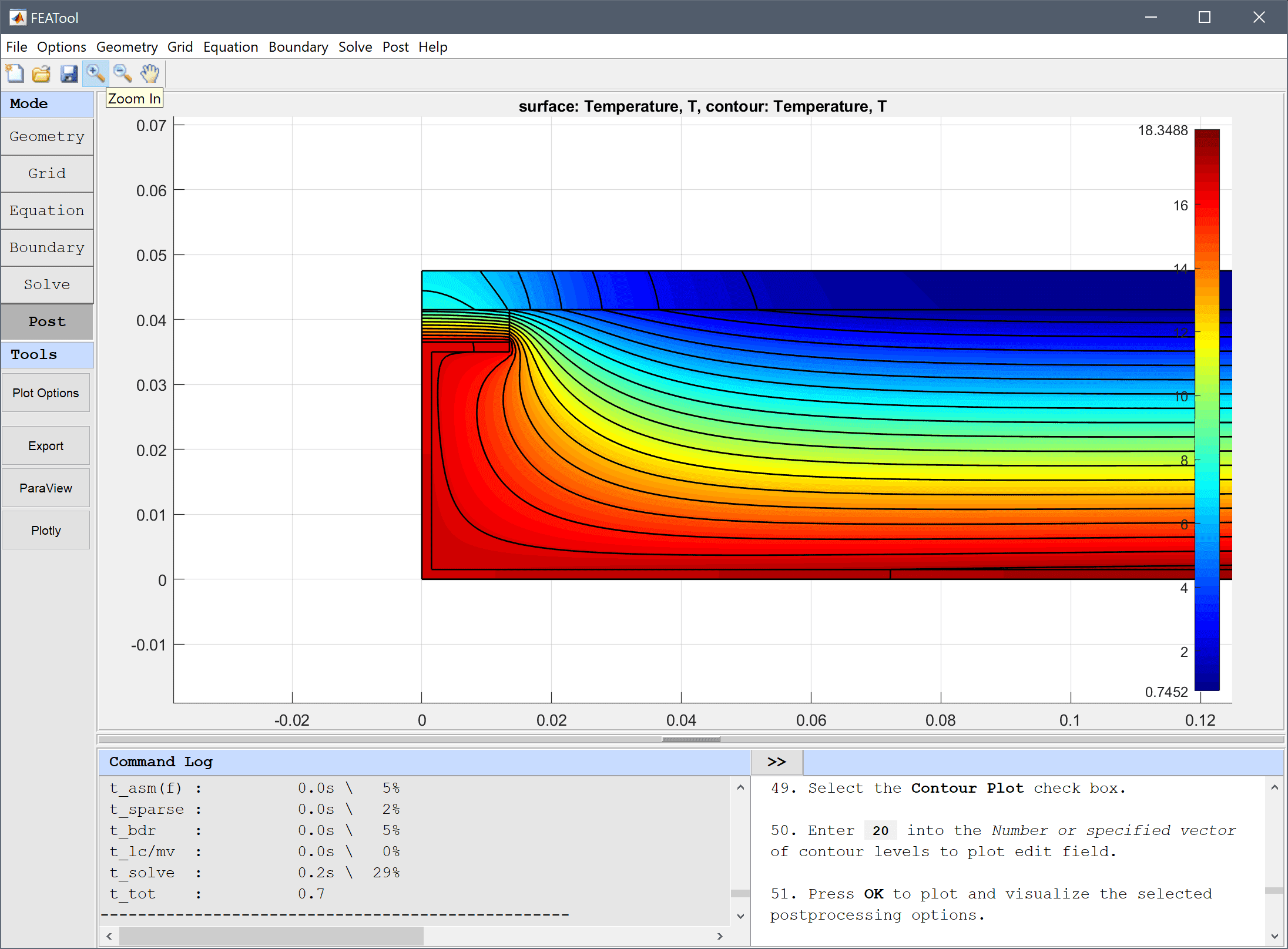
7. Enter 1/0.11 into the Heat transfer coefficient edit field.
8. Enter 20 into the Bulk temperature edit field.
9. Press OK to finish the boundary condition specification.
10. Now that the problem is fully specified, press the Solve Mode Toolbar button to switch to solve mode. Then press the = Tool button to call the solver with the default solver settings.

After the problem has been solved FEATool will automatically switch to postprocessing mode and display the Temperature. Open the postprocessing settings dialog box by clicking on the Plot Options Toolbar button and enable contour plot, as well as zoom in left side to see temperature in the joint section more clearly.

1. Press the Plot Options Toolbar button.
2. Select the Contour Plot check box.
3. Enter 20 into the Number or specified vector of contour levels to plot edit field.

4. Press OK to plot and visualize the selected postprocessing options.

   

Use the boundary integration menu option to calculate the inward and outward normal heat flux.

1. Select Boundary Integration... from the Post menu.
2. Select Normal total heat flux, T from the Predefined integration expressions drop-down menu.
3. Select the bottom boundary, number 1, in the Boundaries list box.
4. Press the Apply button.
5. Then select the top boundary, number 7, in the Boundaries list box.

6. Press the Apply button.

   

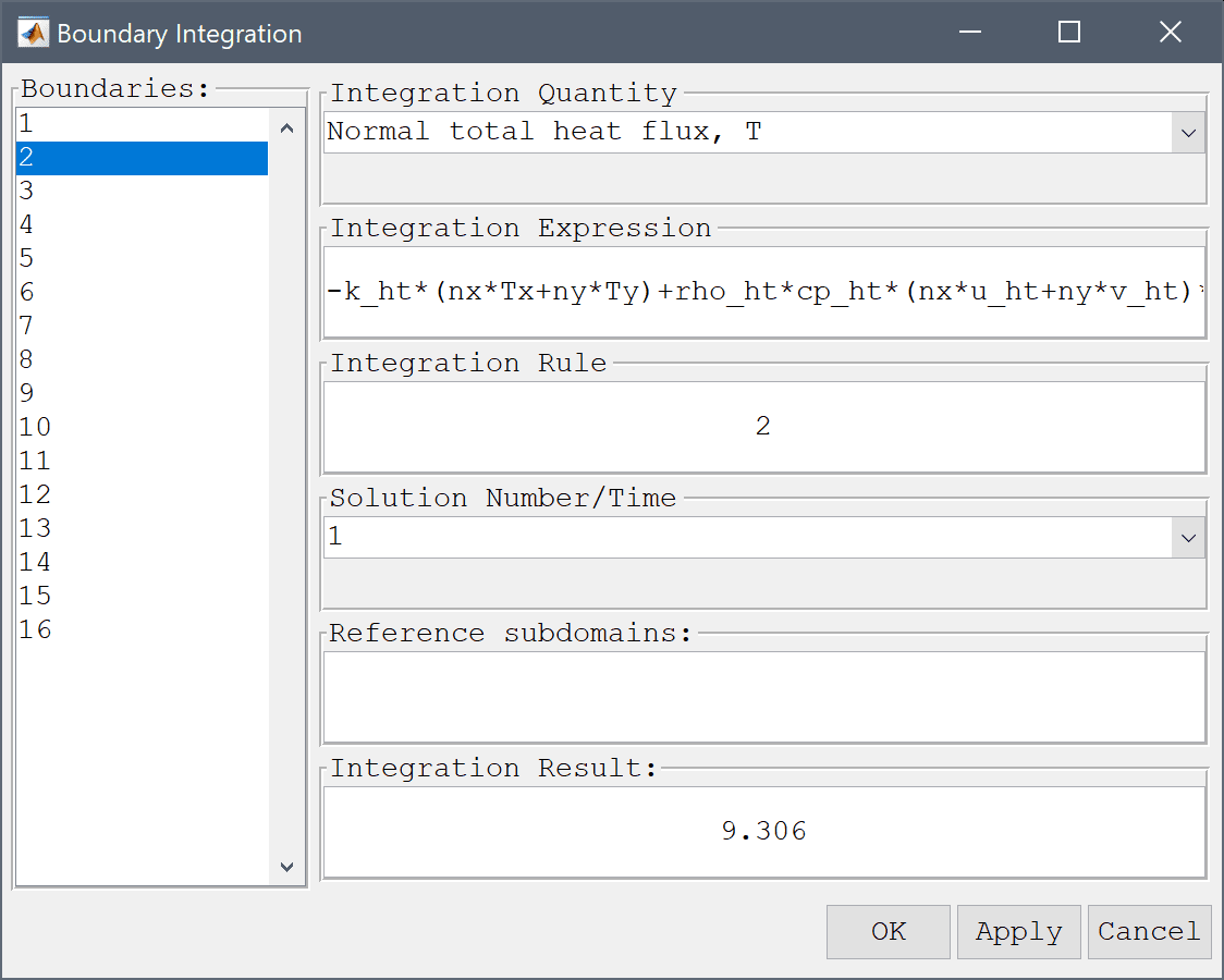
We can see that a negative inward flux from the bottom boundary and corresponding outward from the top (with the convention that normal vectors point outwards). The computed heat flux magnitude of 9.3 compares well with the reference flux value of 9.5 W [1].

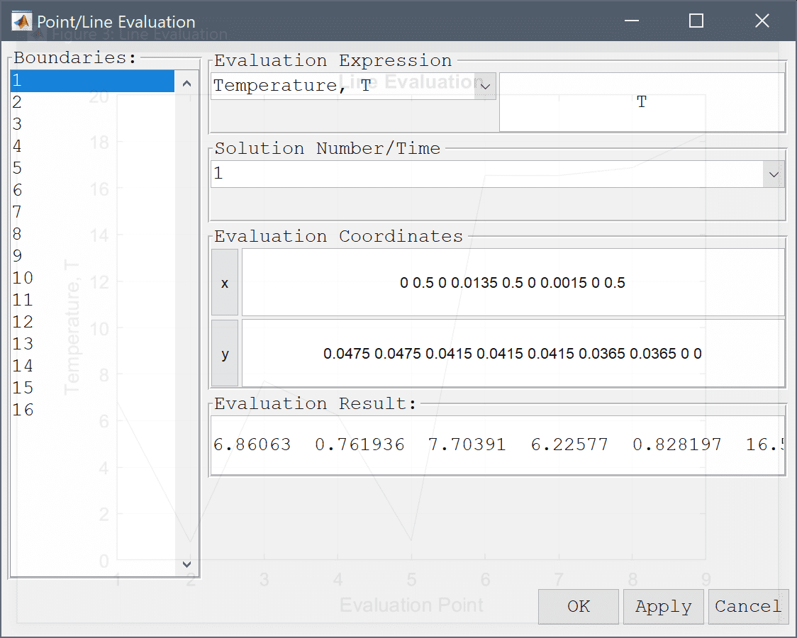
Lastly, we can use the point evalution menu option to compute the temperature and compare with the reference values

x	y	T
0	0.0475	7.1
0.5	0.0475	0.8
0	0.0415	7.9
0.0135	0.0415	6.3
0.5	0.0415	0.8
0	0.0365	16.4
0.0015	0.0365	16.3
0	0	16.8
0.5	0	18.3

1. Press OK to finish and close the dialog box.
2. Select Point/Line Evaluation... from the Post menu.
3. Select Temperature, T from the Evaluation Expression drop-down menu.
4. Enter 0 0.5 0 0.0135 0.5 0 0.0015 0 0.5 into the Evaluation coordinates in x-direction edit field.
5. Enter 0.0475 0.0475 0.0415 0.0415 0.0415 0.0365 0.0365 0 0 into the Evaluation coordinates in y-direction edit field.

6. Press the Apply button.

   
7. Press the Cancel button to close the dialog box.

The thermal bridge heat transfer model has now been completed and can be saved as a binary (.fea) model file, or exported as a programmable MATLAB m-script text file, or GUI script (.fes) file.

Reference

[1] ISO 10211:2007(en), Thermal bridges in building construction - Heat flows and surface temperatures, Test Case A.2.