Cooling Effect of Adding Fins

This example models heated steam at a constant temperature of 120 C flowing through a aluminium pipe with 3 cm diameter. Heat loss to the surrounding cool air (at 25 C and heat transfer coefficient of h = 60 W/m2 C) is computed for a plain pipe, and also a pipe where 200 cooling fins per meter has been added. The simulation results are also compared with theoretical solutions.

Tutorial

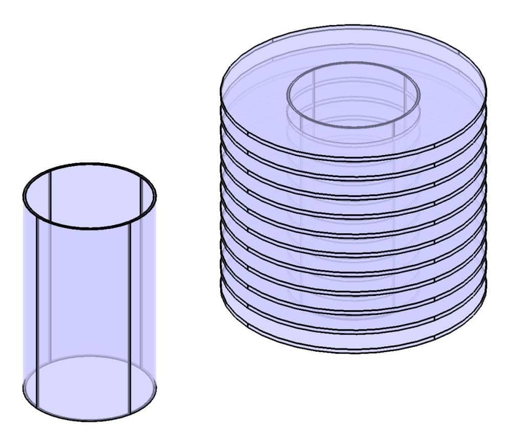
This model is available as an automated tutorial by selecting Model Examples and Tutorials... > Heat Transfer > Cooling Effect of Adding Fins from the File menu. Or alternatively, follow the step-by-step instructions below. Note that the CFDTool interface differ slightly from the FEATool Multiphysics instructions described in the following.

1. To start a new model click the New Model toolbar button, or select New Model... from the File menu.
2. Select the 3D radio button.
3. Select the Heat Transfer physics mode from the Select Physics drop-down menu. (Note that for CFDTool the physics selection is done in the Equation settings dialog box.)

4. Press OK to finish the physics mode selection.

   

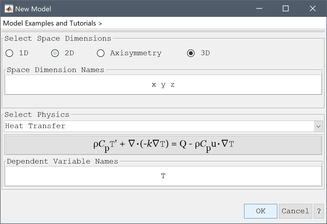
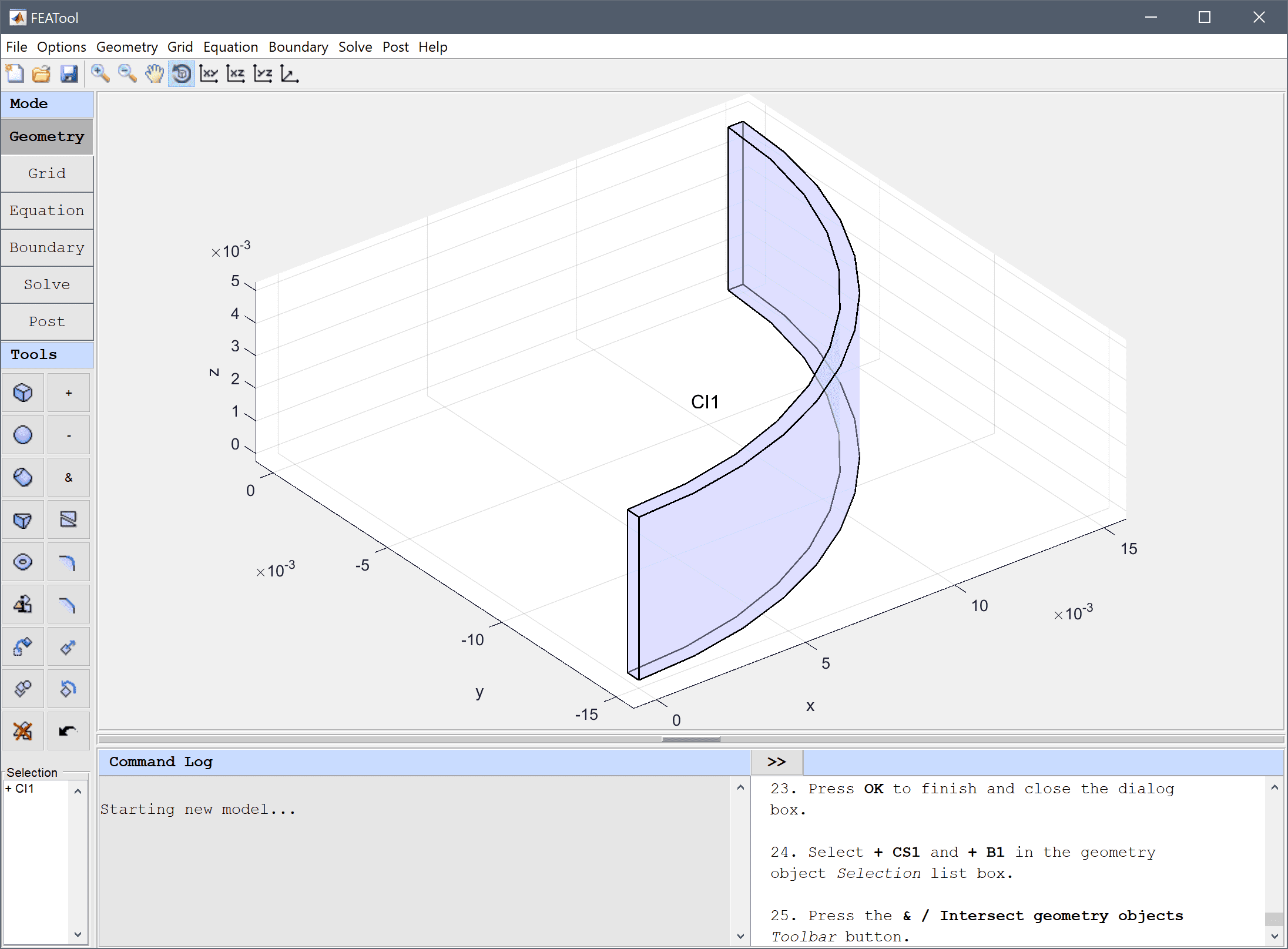
Due to symmetry it is sufficient to model a small section, here taken as quarter section of length 5 mm (this model would also be possible to reduce to 2D axisymmetry).

1. Press the Create cylinder/cone Toolbar button.
2. Enter 0.015 into the radius₁ edit field.
3. Enter 0.015 into the radius₂ edit field.
4. Enter 1/200 into the length edit field.
5. Enter 0 0 1 into the axis edit field.
6. Press OK to finish and close the dialog box.
7. Press the Create cylinder/cone Toolbar button.
8. Enter 0.0145 into the radius₁ edit field.
9. Enter 0.0145 into the radius₂ edit field.
10. Enter 1/200 into the length edit field.
11. Enter 0 0 1 into the axis edit field.
12. Press OK to finish and close the dialog box.
13. Select C1 and C2 in the geometry object Selection list box.
14. Press the - / Subtract geometry objects Toolbar button.

Then create a block overlapping a quarter and intersect it with the resulting cylindrical pipe shell.

1. Press the Create cube/block Toolbar button.
2. Enter 0.015 into the x_max edit field.
3. Enter -0.015 into the y_max edit field.
4. Enter 1/200 into the z_max edit field.
5. Press OK to finish and close the dialog box.
6. Select CS1 and B1 in the geometry object Selection list box.

7. Press the & / Intersect geometry objects Toolbar button to crete the final geometry shape.

   
8. Switch to Grid mode by clicking on the corresponding Mode Toolbar button.

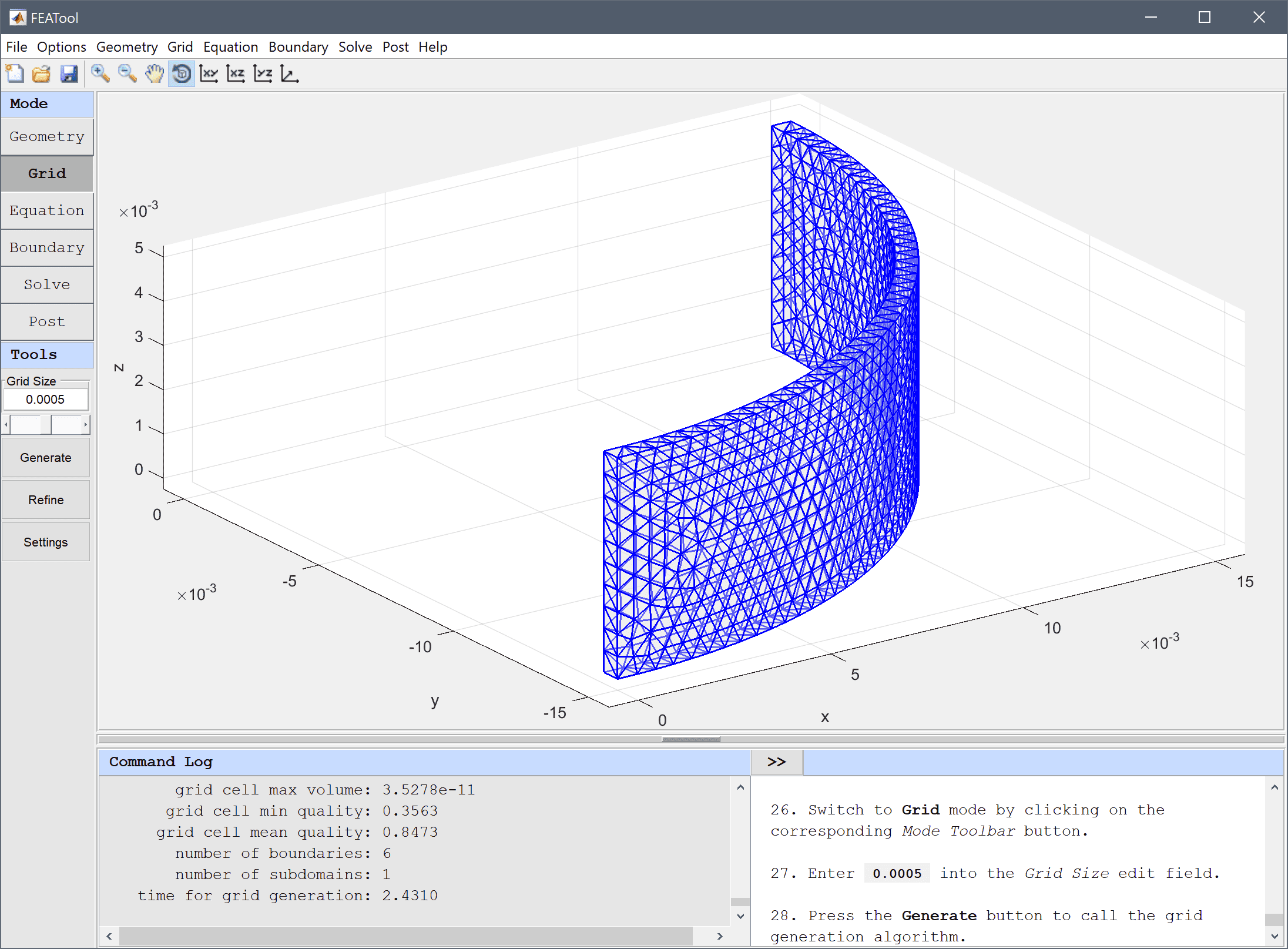
9. Enter 0.0005 into the Grid Size edit field and press the Generate button to call the grid generation algorithm.

   
10. Switch to Equation mode by clicking on the corresponding Mode Toolbar button.

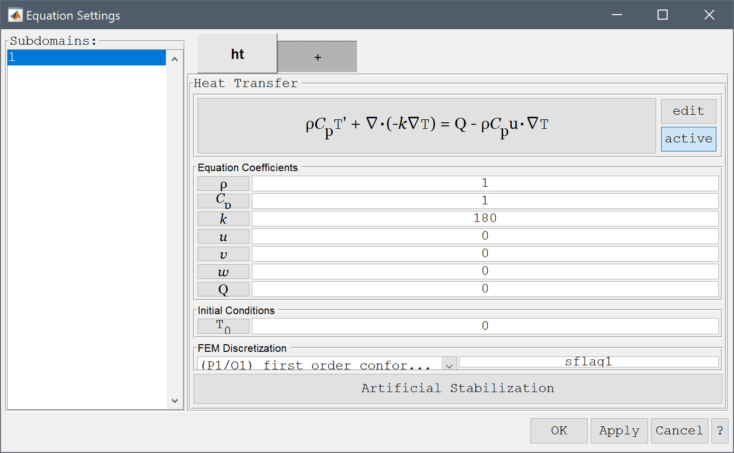
11. In the Equation Settings dialog box, set the thermal conductivity to 180 W/m C, the other coefficients will not be used, they can be left to their default values. Note that it is up to the user to define and use a consistent system of units for coefficients and parameters, here SI units is chosen. (Note that the Equation Settings dialog box may look different for CFDTool.)

    
12. Press OK to finish the equation and subdomain settings specification.
13. Switch to Boundary mode by clicking on the corresponding Mode Toolbar button.
14. Set the temperature to 120 C for the inner boundary.

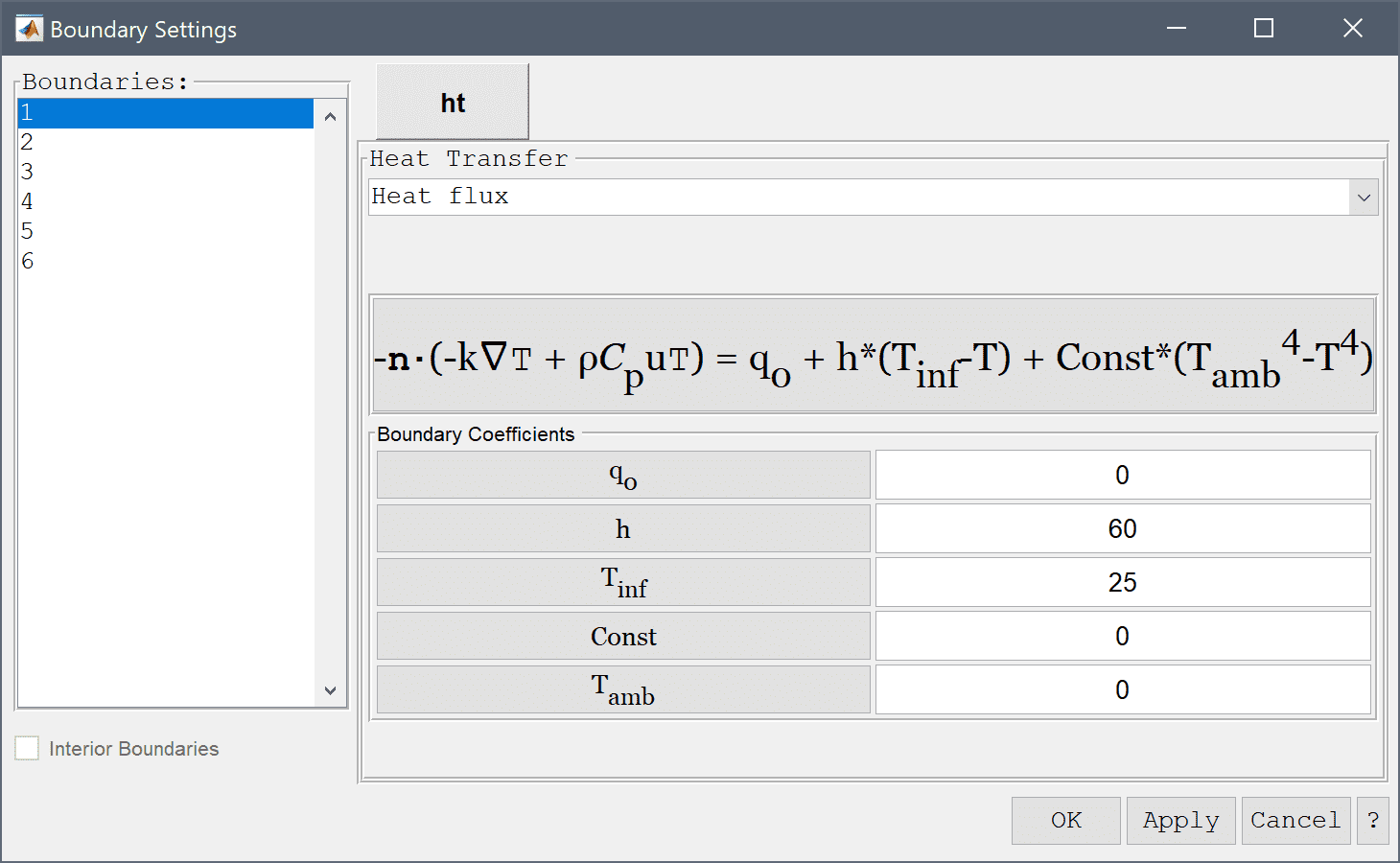
15. The Heat flux condition should be selected for the outer boundary, with a heat transfer coefficient 60 W/m C and surrounding bulk temperature of 25 C. This condition prescribes the rate at which heat is lost to the surrounding air (which is not modeled here).

    
16. Select Thermal insulation/symmetry for the rest of the boundaries. This condition is appropriate for boundaries that in reality are extended symmetrically as here.
17. Press OK to finish the boundary condition specification.
18. Switch to Solve mode by clicking on the corresponding Mode Toolbar button.
19. Press the = Toolbar button to call the solver. After the problem has been solved FEATool will automatically switch to postprocessing mode and plot the computed solution.

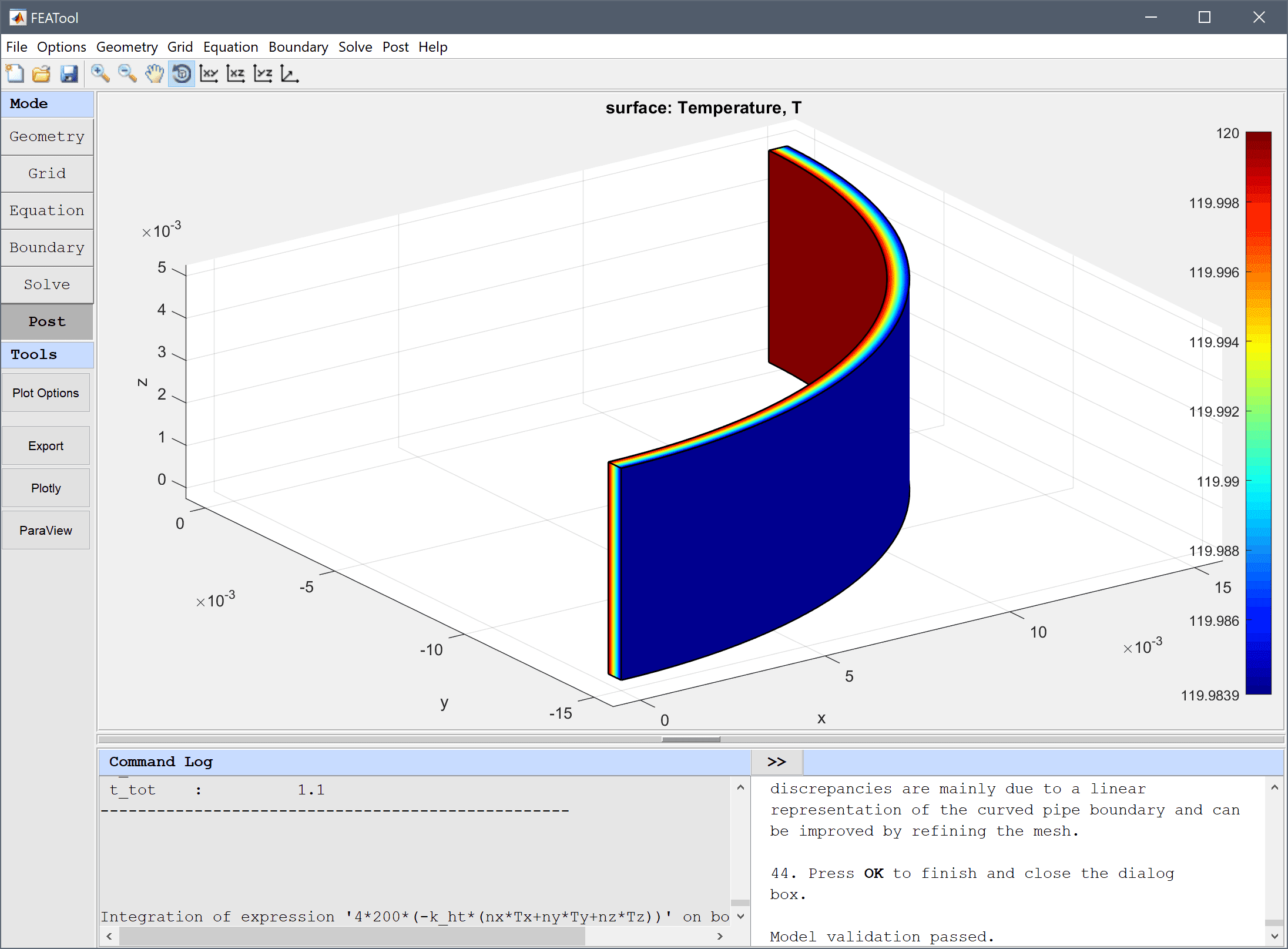
After the problem has been solved FEATool will automatically switch to postprocessing mode and show the computed Temperature where we can see that the outside of the pipe has been somewhat cooled due to heat loss.

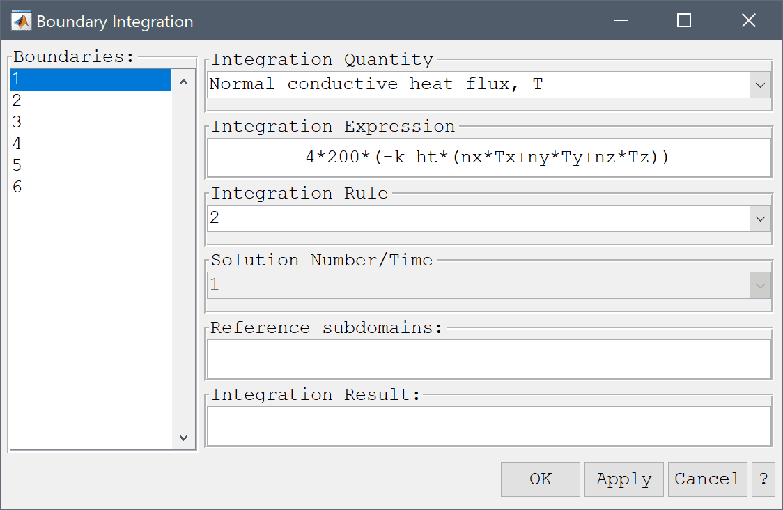
We also can calculate the computed heat loss by integrating the heat flux on the outer boundary and compare it with the theoretical solution.

1. Select Boundary Integration... from the Post menu.
2. Select the outer boundary (here 1) in the Boundaries list box.
3. Select Normal conductive heat flux, T from the Predefined integration expressions drop-down menu.

Multiply the expression for the outward heat flux with 4*200 (accounting for simulation of a 5 mm quarter section) to get the total heat loss in W/m.

1. Enter 4*200*(-k_ht*(nx*Tx+ny*Ty+nz*Tz)) into the Integration Expression edit field.

The computed value should be close to the theoretical reference value of 537 W/m. The small discrepancies are mainly due to a linear representation of the curved pipe boundary and can be improved by refining the mesh.

1. Press OK to finish and close the dialog box, the resulting integrand should be printed in the output and message log.

To compare the heat loss with the modified geometry, first go back to Geometry mode to add the fins.

1. Switch to Geometry mode by clicking on the corresponding Mode Toolbar button.

Use the undo geometry objects button to recover the original input shapes.

1. Select CI1 and CS1 in the geometry object Selection list box.
2. Then press the Undo/revert modified/transformed geometry object(s) Toolbar button.

Now two cylinders for the fins should be added to the top and bottom of the pipe.

1. Press the Create cylinder/cone Toolbar button.
2. Enter 0.03 into the radius₁ edit field.
3. Enter 0.03 into the radius₂ edit field.
4. Enter 1e-3 into the length edit field.
5. Enter 0 0 1 into the axis edit field.
6. Press OK to finish and close the dialog box.
7. Press the Create cylinder/cone Toolbar button.
8. Enter 0 0 into the center edit field.
9. Enter 0 0 1/200-1e-3 into the center edit field.
10. Enter 0.03 into the radius₁ edit field.
11. Enter 0.03 into the radius₂ edit field.
12. Enter 1e-3 into the length edit field.
13. Enter 0 0 1 into the axis edit field.
14. Press OK to finish and close the dialog box.

Extend the block to also cover the fins.

1. Select B1 in the geometry object Selection list box.
2. To modify and edit the selected geometry object, click on the Inspect/edit selected geometry object Toolbar button to open the Edit Geometry Object dialog box.
3. Enter 0.03 into the x_max edit field.
4. Enter -0.03 into the y_min edit field.
5. Press OK to finish and close the dialog box.

Finally join the outer cylinder and fins, subtract the inner cylinder, and intersect with the block to generate the final shape.

1. Select Combine Objects... from the Geometry menu.

2. Enter C1 + C3 + C4 - C2 & B1 into the Geometry Formula edit field.

   
3. Press OK to finish and close the dialog box.
4. Switch to Grid mode by clicking on the corresponding Mode Toolbar button.

5. Enter 0.0005 into the Grid Size edit field and press the Generate button to generate a mesh for the modified geometry.

   

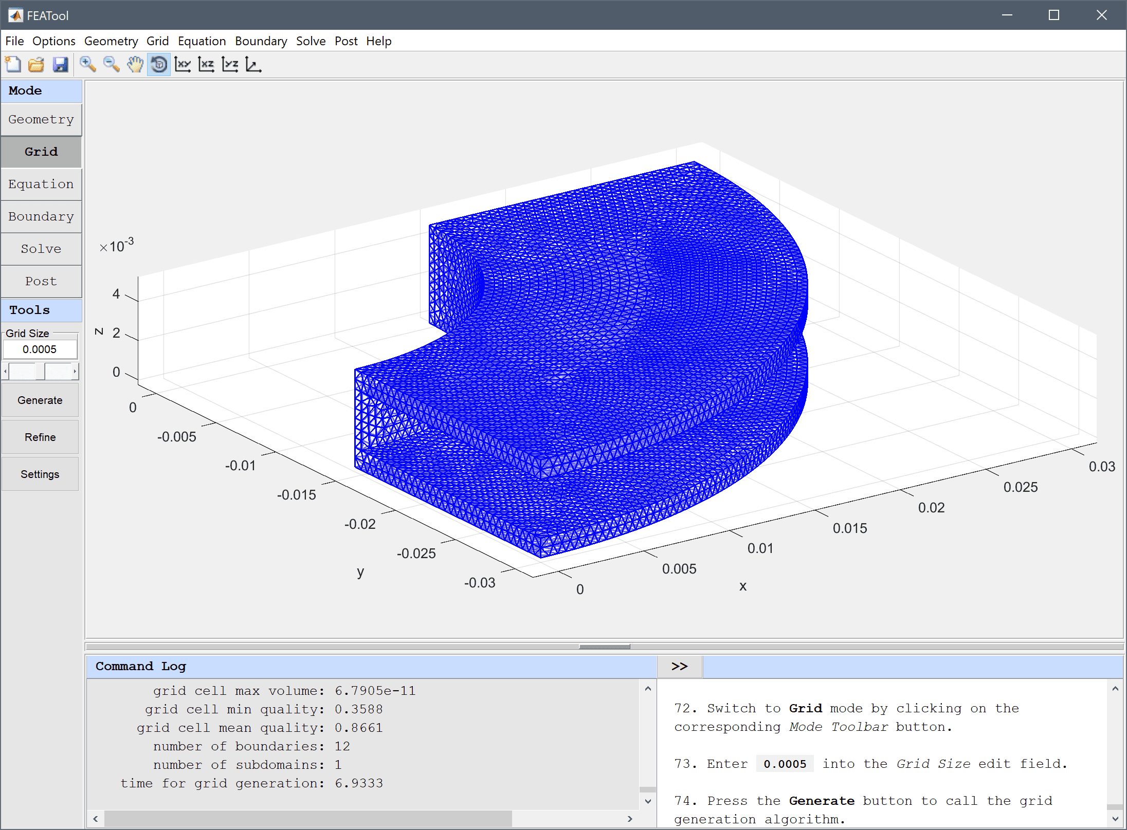
Set the boundary conditions similar to the first simulation with the original shape (with the difference that there now are more boundary segments due to the added fins).

1. Switch to Boundary mode by clicking on the corresponding Mode Toolbar button.
2. Select the inner boundary (3) in the Boundaries list box.
3. Select Temperature from the Heat Transfer drop-down menu.
4. Enter 120 into the Temperature edit field.
5. Select 1, 2, and 4-7 in the Boundaries list box.
6. Select Thermal insulation/symmetry from the Heat Transfer drop-down menu.
7. Select 8-12 in the Boundaries list box.
8. Select Heat flux from the Heat Transfer drop-down menu.
9. Enter 60 into the Heat transfer coefficient edit field, and 25 into the Bulk temperature edit field.
10. Press OK to finish the boundary condition specification.
11. Switch to Solve mode by clicking on the corresponding Mode Toolbar button.
12. Press the = Toolbar button to call the solver. After the problem has been solved FEATool will automatically switch to postprocessing mode and plot the computed solution.

After solving we can clearly see how the fins help to cool the outer temperature.

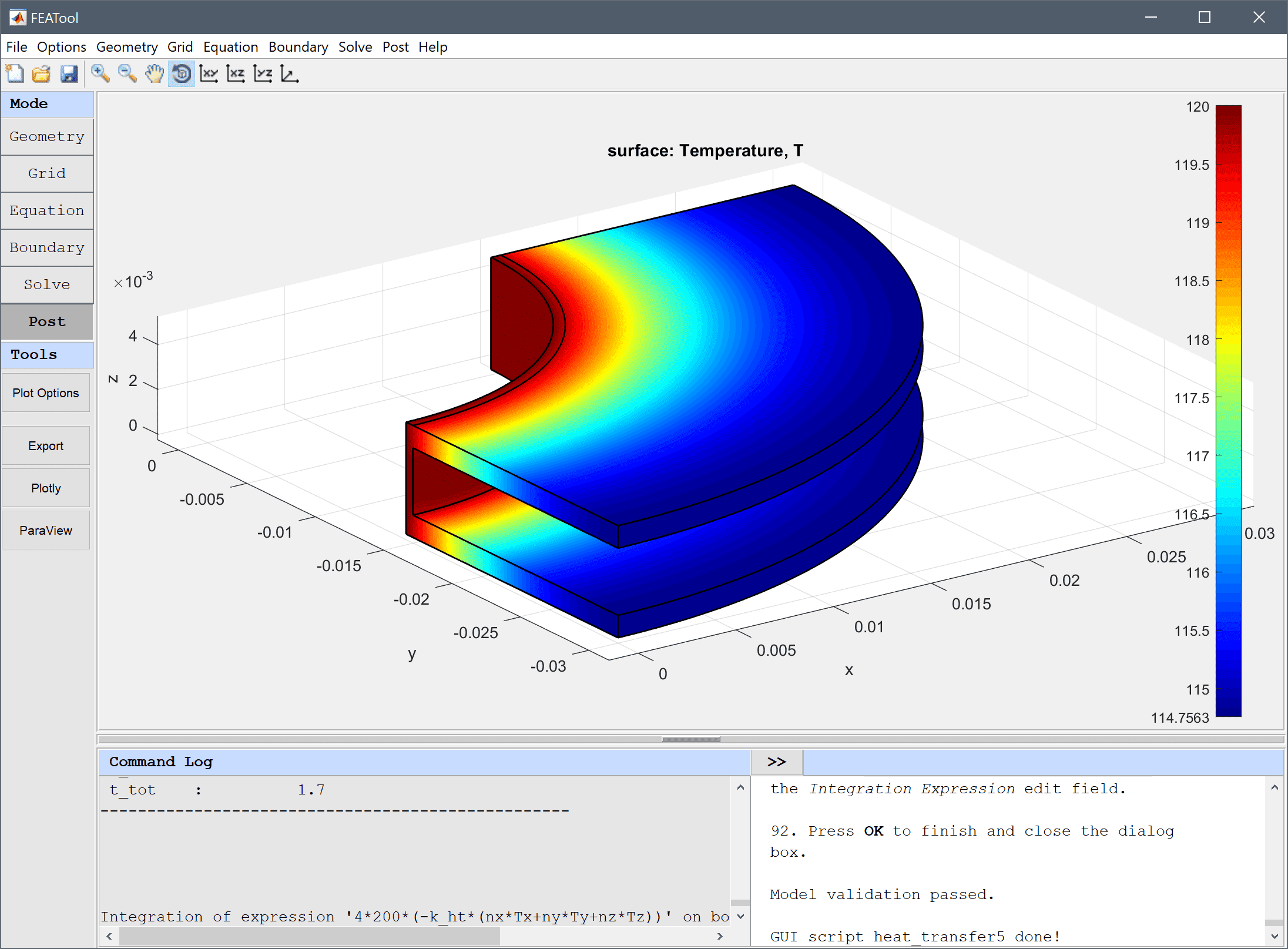
Perform boundary integration of the heat flux as before and compare with the theoretical result 5320 W/m, and note that with the added fins we now get almost 10 times more effective cooling due to the increased added surface area.

1. Select Boundary Integration... from the Post menu.
2. Select boundaries 8-12 in the Boundaries list box.
3. Select Normal conductive heat flux, T from the Predefined integration expressions drop-down menu.
4. Enter 4*200*(-k_ht*(nx*Tx+ny*Ty+nz*Tz)) into the Integration Expression edit field.
5. Press OK to finish and close the dialog box, the resulting integrand should be printed in the output and message log.

The cooling effect of adding fins heat transfer model has now been completed and can be saved as a binary (.fea) model file, or exported as a programmable MATLAB m-script text file, or GUI script (.fes) file.

Reference

[1] Cengel, Yunus A., Heat Transfer: A Practical Approach, WCB/McGraw-Hill, 1998.