Heat Conduction with Tabulated Thermal Conductivity

This heat conduction tutorial example illustrates how to use data from a (text) file in an equation coefficient. The tabulated data here represents non-linear thermal conductivity as a function of temperature k = f(T). Where the conductivity curve is given as sin(pi/8) to sin(3/4*pi) for temperature values between 280 to 400. In the data (text) file the first column represents temperature values and second the coefficient value:

280.0000 0.3827
281.2121 0.4009
...
398.7879 0.7210
400.0000 0.7071

The coefficient is implemented and called from the toolbox using the finterpn function, which also supports interpolation in higher n dimensions (as well as csv and mat file formats).

Tutorial

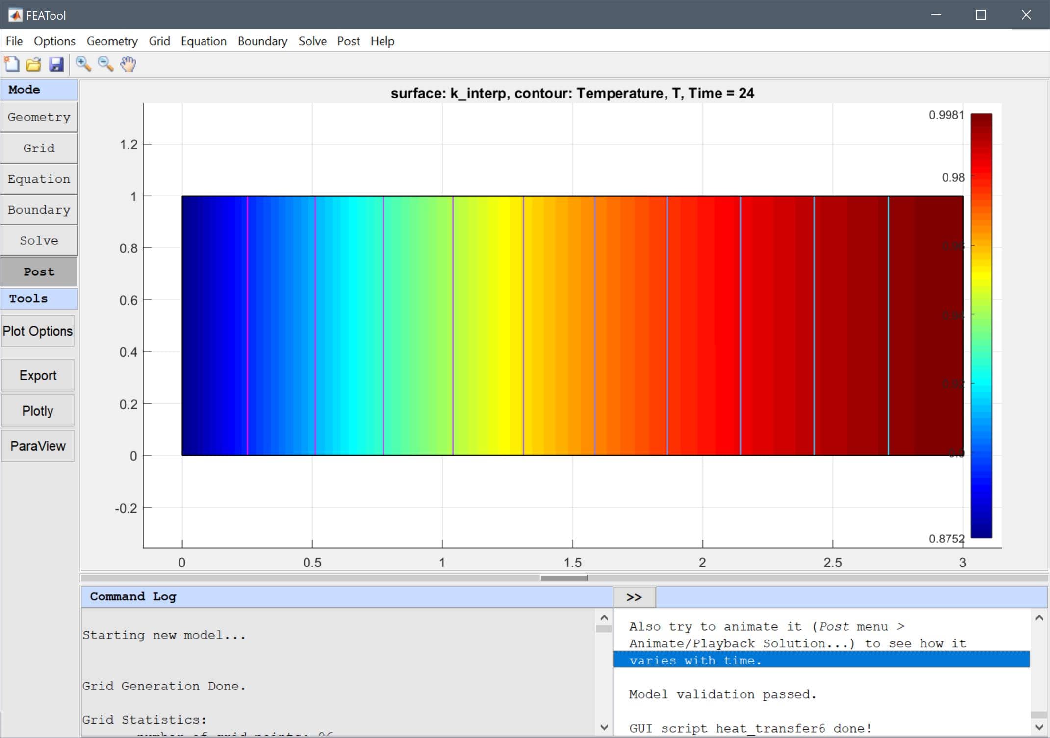
This model is available as an automated tutorial by selecting Model Examples and Tutorials... > Heat Transfer > Heat Conduction with Tabulated Thermal Conductivity from the File menu. Or alternatively, follow the step-by-step instructions below. Note that the CFDTool interface differ slightly from the FEATool Multiphysics instructions described in the following.

1. To start a new model click the New Model toolbar button, or select New Model... from the File menu.
2. Select the Heat Transfer physics mode from the Select Physics drop-down menu.
3. Press OK to finish the physics mode selection.

The simple geometry consists of 3 x 1 rectangle, and a mesh with a 0.05 grid cell diameter.

1. Select Rectangle from the Geometry menu.
2. Enter 3 into the x_max edit field.
3. Press OK to finish and close the dialog box.
4. Switch to Grid mode by clicking on the corresponding Mode Toolbar button.
5. Enter 0.05 into the Grid Size edit field.
6. Press the Generate button to call the grid generation algorithm.
7. Switch to Equation mode by clicking on the corresponding Mode Toolbar button.
8. In the Equation Settings dialog box, set the coefficient of Thermal Conductivity to k_interp (to be defined later), and the initial temperature to 300.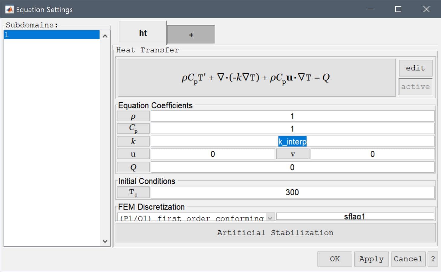

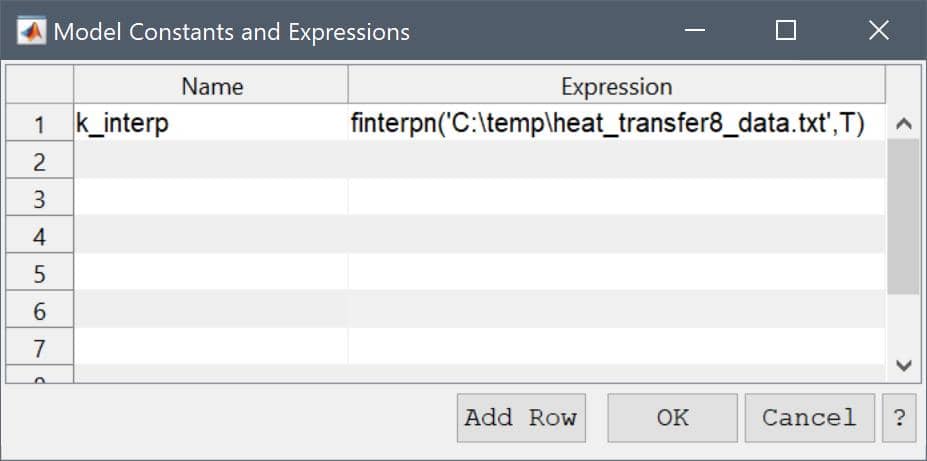
1. Press OK to finish the equation and subdomain settings specification.

Now add an equation expression named k_interp, with the value finterpn('heat_transfer8_data.txt',T). Where the file heat_transfer8_data.txt contains the tabulated data data = [linspace(280,420)', sin(linspace(pi/8,3/4*pi,100))'] to be interpolated. When evaluated this coefficient will call the finterpn function which reads the data from the file, interpolates, and returns the result.

1. Execute the following commands on the MATLAB command line to generate the data file (including the full path to the file), or create it manually through other means

   data = [linspace(280,420)', sin(linspace(pi/8,3/4*pi,100))'];
   save('heat_transfer8_data.txt', '-ascii', 'data')
   

2. Press the Constants Toolbar button.

Enter k_interp into row and column (1, 1), and finterpn('heat_transfer8_data.txt',T) into row and column (1, 2) of the table.

1. Press OK to finish and close the dialog box.
2. Switch to Boundary mode by clicking on the corresponding Mode Toolbar button.

In boundary mode, first set the top and bottom boundaries to Thermal insulation/symmetry.

1. Select 1 and 3 in the Boundaries list box.
2. Select Thermal insulation/symmetry from the Heat Transfer drop-down menu.

The right boundary features a negative heat flux -10.

1. Select 2 in the Boundaries list box.
2. Select Heat flux from the Heat Transfer drop-down menu.
3. Enter -10 into the Inward heat flux edit field.

And the left boundary a fixed temperature of 400.

1. Select 4 in the Boundaries list box.
2. Select Temperature from the Heat Transfer drop-down menu.
3. Enter 400 into the Temperature edit field.
4. Press OK to finish the boundary condition specification.
5. Switch to Solve mode by clicking on the corresponding Mode Toolbar button.

In the Solver Settings dialog box, select the Time-Dependent solver, a time step of 0.5, and 100 maximum time steps.

1. Press the Settings Toolbar button.
2. Select Time-Dependent from the Solution and solver type drop-down menu.
3. Enter 0.5 into the Time step size edit field.
4. Enter 100 into the Duration of time-dependent simulation (maximum time) edit field.

The tstop parameters will stop the simulation if the normed differences between time-steps is 1e-4 or lower, assuming a stationary state has been reached.

1. Enter 1e-4 into the Stopping criteria for solution differences (changes) between time steps edit field.
2. Press OK to apply the selected solver settings.
3. Press the = Toolbar button to call the solver. After the problem has been solved the toolbox will automatically switch to postprocessing mode and plot the computed solution.

Note that the solver stopped after 24 seconds, as the tstop condition has been fulfilled.

Open the Postprocessing Settings dialog box and plot the thermal conductivity k_interp to see how it varies with temperature.

1. Press the Plot Options Toolbar button.
2. Enter k_interp into the Surface plot expression edit field.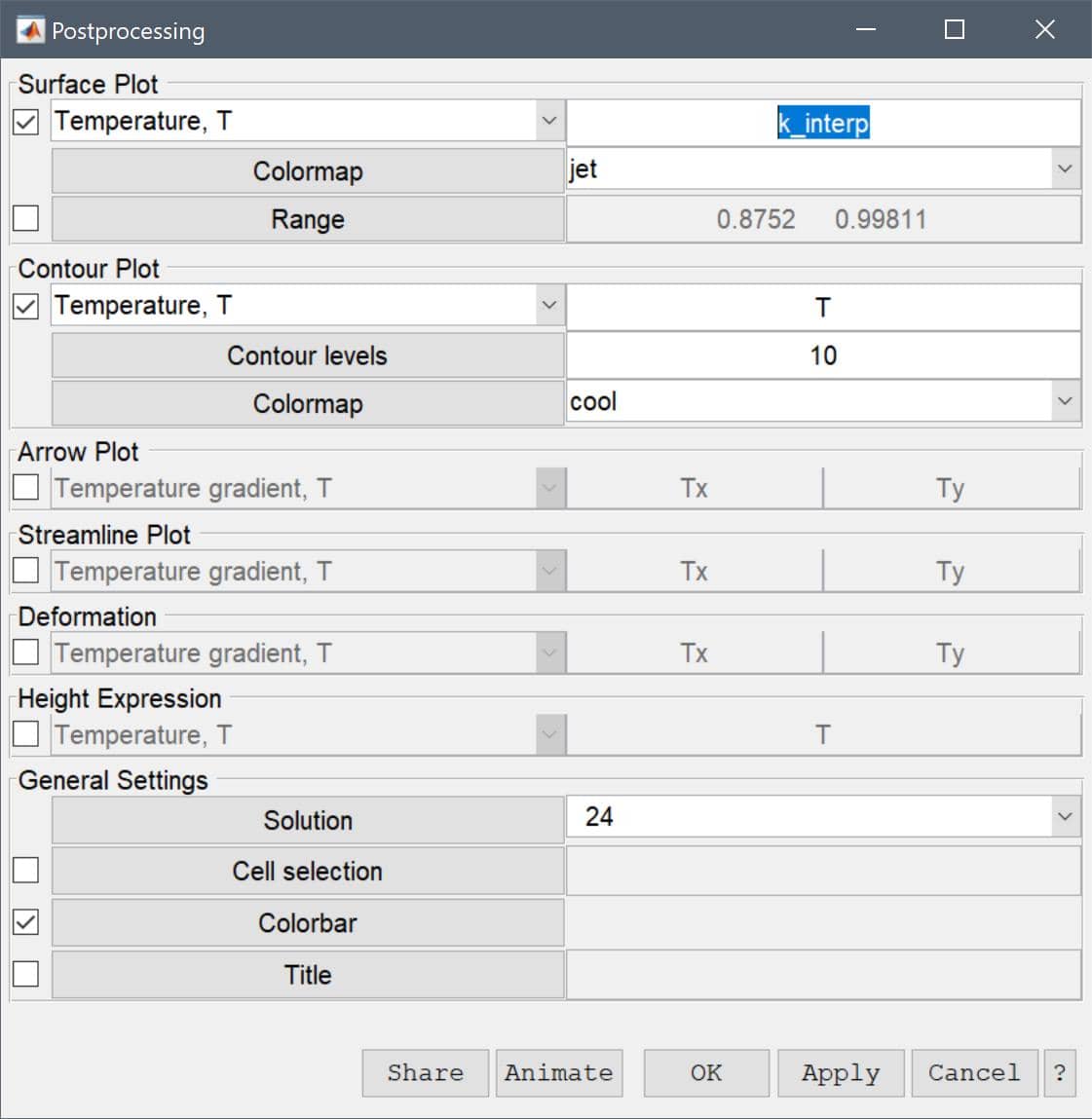
3. Select the Enable/disable contour plot check box to plot the temperature field T as contour lines.

1. Press OK to plot and visualize the selected postprocessing options.

Also try to animate it (Post menu > Animate/Playback Solution...) to see how it varies with time.

The heat conduction with tabulated thermal conductivity heat transfer model has now been completed and can be saved as a binary (.fea) model file, or exported as a programmable MATLAB m-script text file, or GUI script (.fes) file.