This example shows how to model a battery pack stacked with 20 prismatic battery cells. A heat transfer analysis will be conducted for the model where it is assumed that one of the battery cells is faulty resulting in significantly increased heat generation in the cell.

Two different cases will be studied, one where the pack is perfectly insulated, except for the front and back faces which are cooled through natural convection with the surrounding air. And also a second case study with added increased cooling at the bottom of the battery pack.

The example tutorial highlights the following features:

3D CAD STEP geometry import
Heat transfer simulation with convective cooling
Anisotropic material coefficients (thermal conductivity) and using different material properties in different subdomains
Solution restart (using a previously computed data)
Evaluation and analysis in given evaluation points

Tutorial

This model is available as an automated tutorial by selecting Model Examples and Tutorials... > Heat Transfer > Cooling Analysis of a Battery Pack Module from the File menu. Or alternatively, follow the step-by-step instructions below.

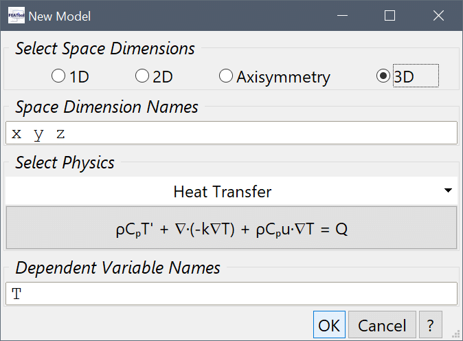
To start a new model click the New Model toolbar button, or select New Model... from the File menu.
Select the 3D radio button, and the Heat Transfer physics mode from the Select Physics drop-down menu. Then press OK to finish the physics mode selection.

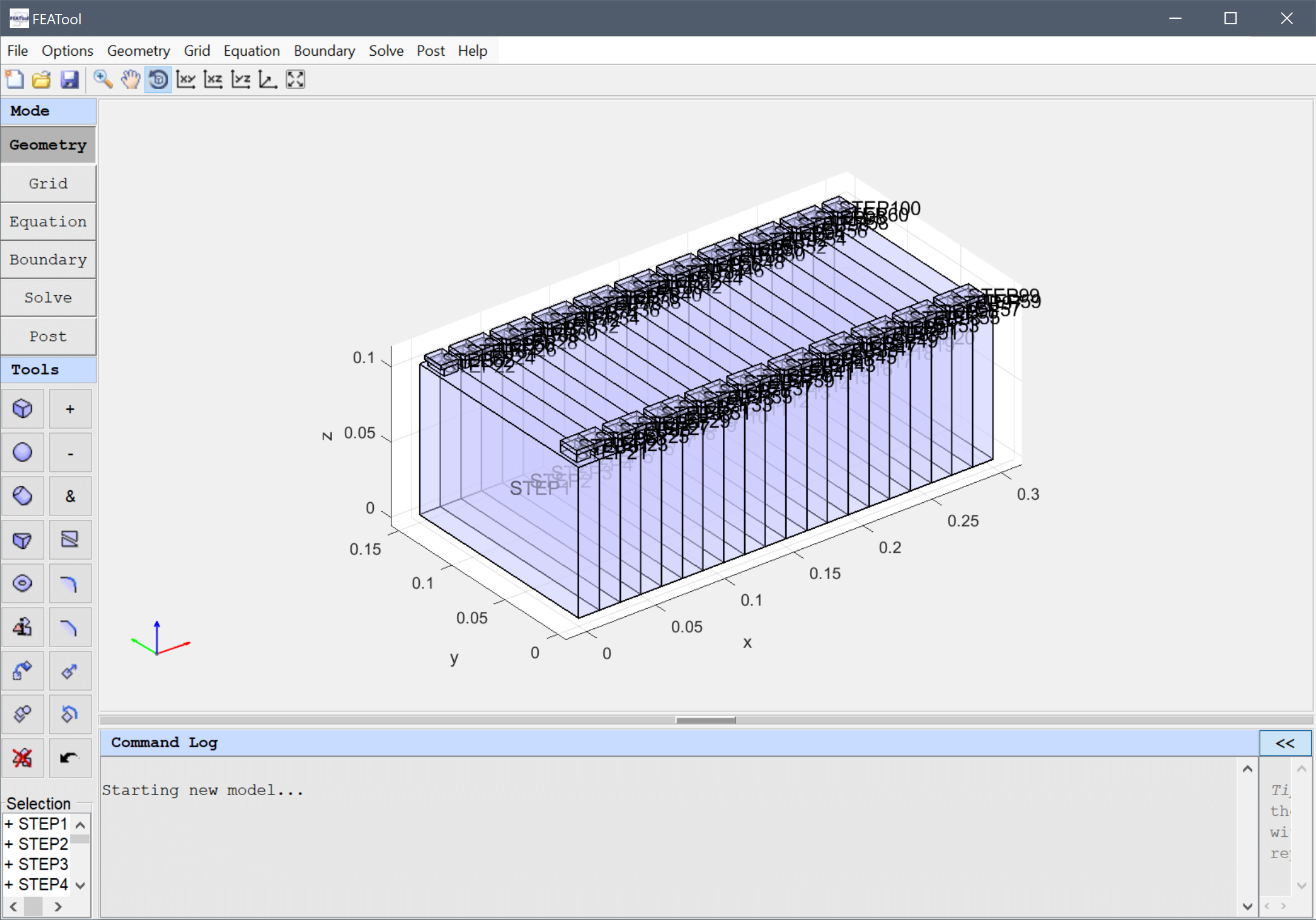
Although the geometry can be generated with the built-in CAD tools, in this case we will import the geometry from a STEP CAD file. (This file can be found as /tutorials/02_Heat_Transfer/battery_pack.step of the toolbox distribution folder.)

Select STEP Format... from the Geometry menu, and select the file to import.
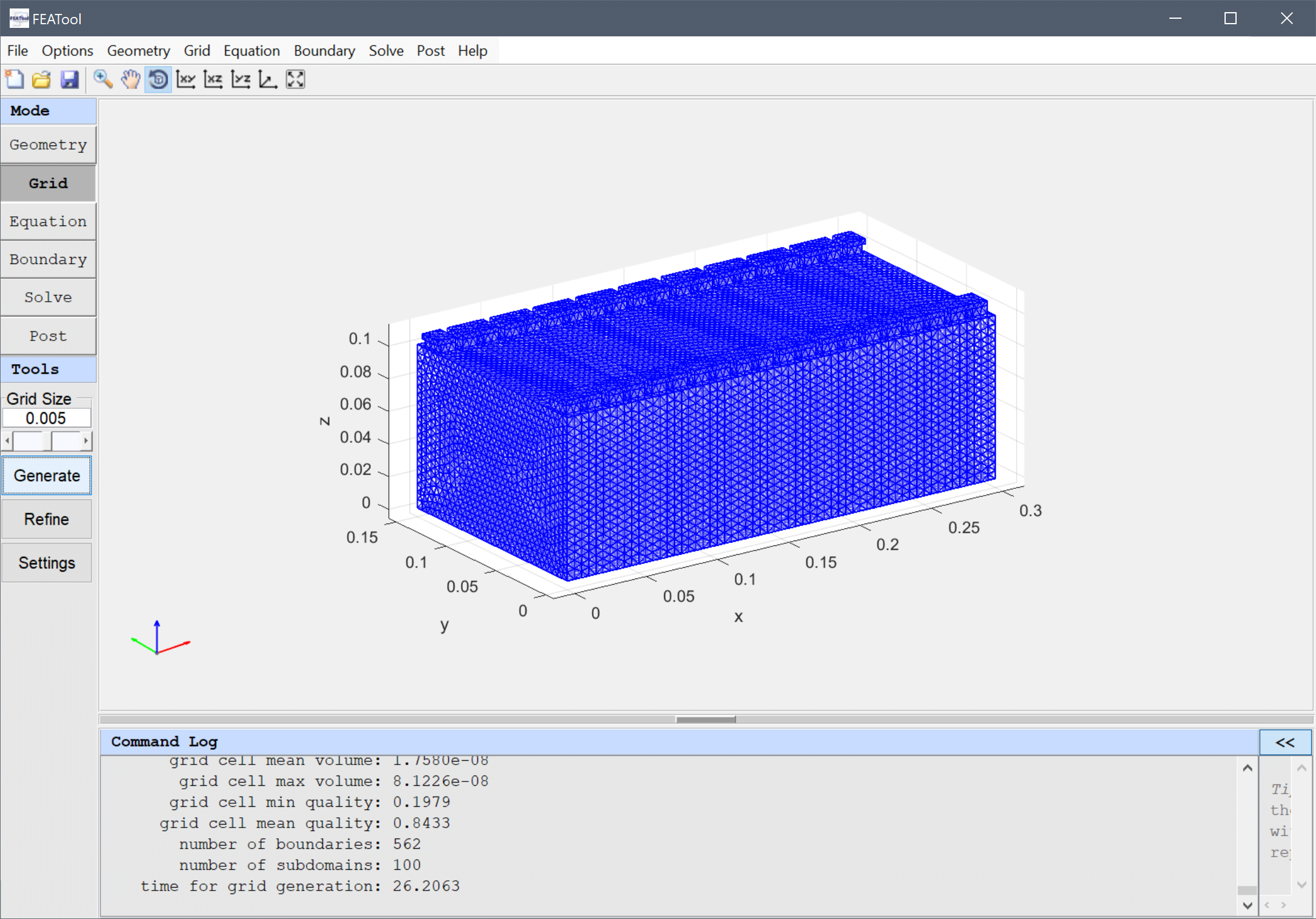
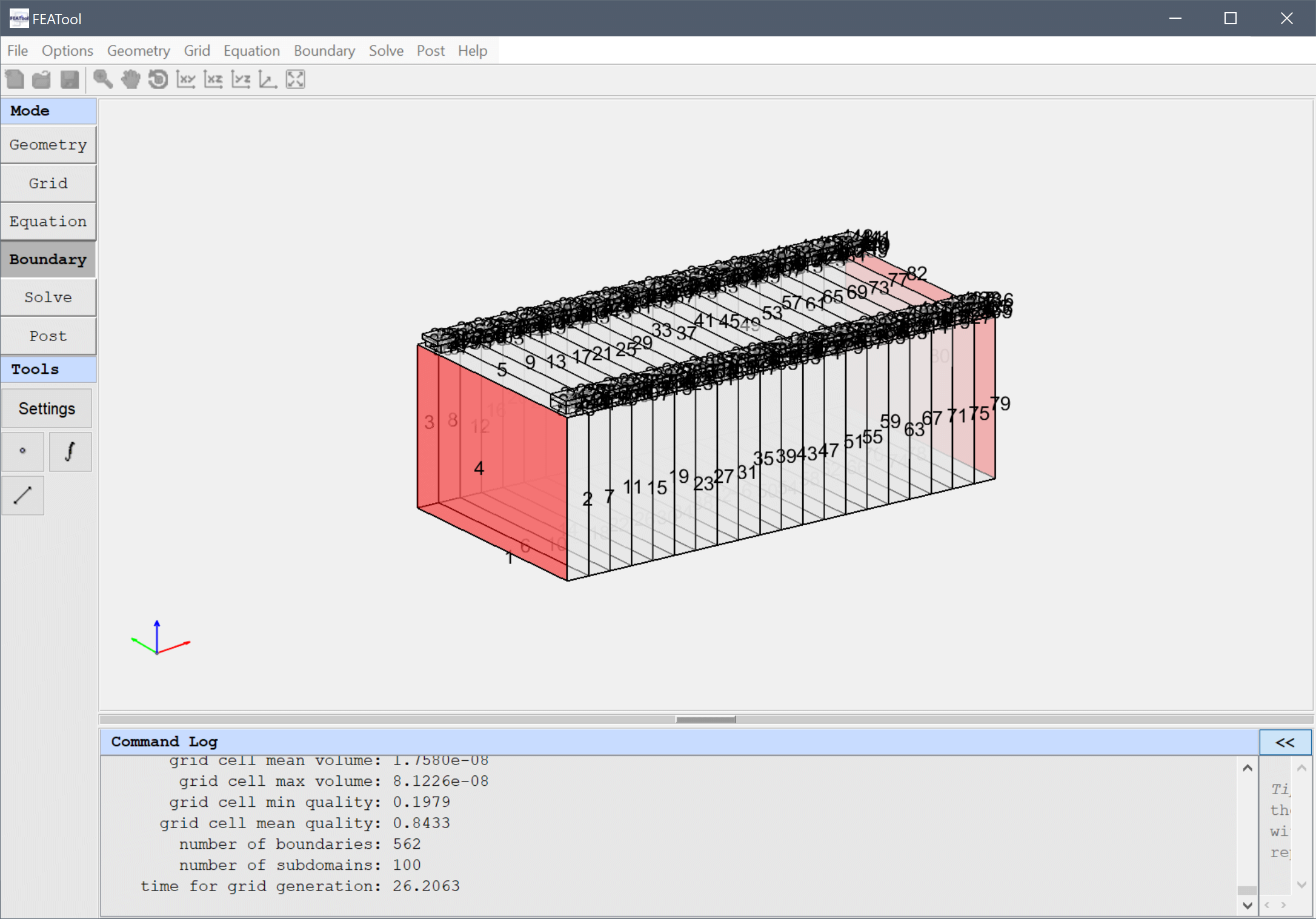
To generate a mesh, first switch to Grid mode by clicking on the corresponding Mode Toolbar button.
Enter 0.005 into the Grid Size edit field, and press the Generate button to call the grid generation algorithm.
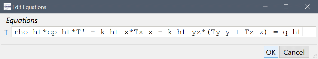
Switch to Equation mode by clicking on the corresponding Mode Toolbar button.

To account for the effect that battery cell walls conduct heat poorly between adjacent cells (even when stacked right next to each other), we will model this as an anisotropic thermal conductivity. That is, heat transfer in the x-direction is poor, while normal in the y/z in-plane directions. To do this we will change the heat diffusion term from isotropic k_ht*(Tx_x + Ty_y + Tz_z), to anisotropic k_ht_x*Tx_x + k_ht_yz*(Ty_y + Tz_z)

To change the equation, press the edit button and enter rho_ht*cp_ht*T' - k_ht_x*Tx_x - k_ht_yz*(Ty_y + Tz_z) = q_ht into the Equation for T edit field (note that the connective term has been omitted as it does not contribute in this simulation). Press OK to finish and close the dialog box.

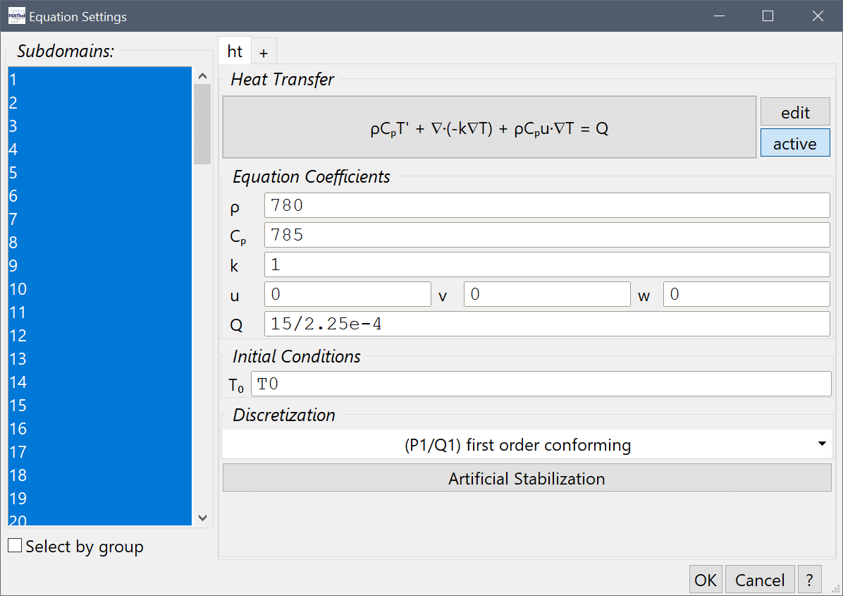
Specify the material parameters for the battery cells.

Select subdomains 1-20 in the Subdomains list box.
Enter 780 into the Density, ρ [kg/m³] edit field, 785 into the Heat capacity, C_p [J/(kg*K)] edit field, and prescribe a Heat source, Q of 15/2.25e-4 [W/m³].

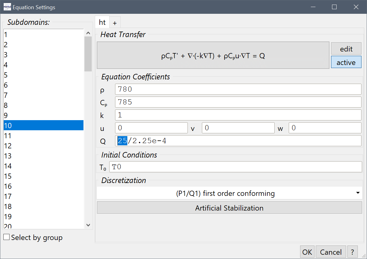
Give the faulty cell (number 10) a higher heat source.

Select 10 in the Subdomains list box, and Enter 25/2.25e-4 into the Heat source, Q edit field.

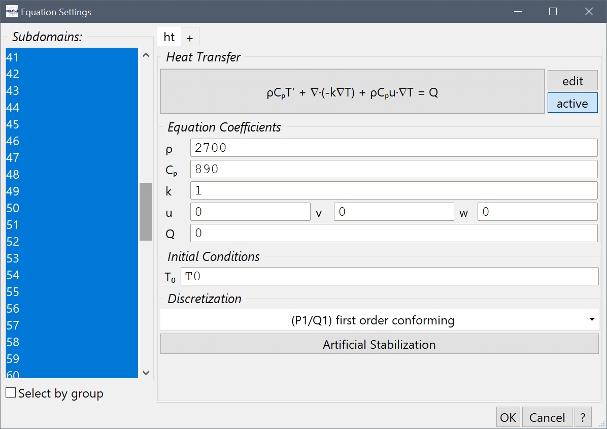
Set the density and heat capacity for the battery tabs (here subdomains 21-60).

Select 21-60 in the Subdomains list box.
Enter 2700 into the Density edit field, and 890 into the Heat capacity edit field.

For the battery connectors (here subdomains 61-100), set the density and heat capacity for 540 and 840, respectively.

Select 61-100 in the Subdomains list box.
Enter 540 into the Density edit field, and 840 into the Heat capacity edit field.

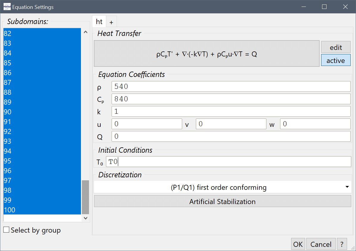
Finally, select all domains and set the initial temperature T₀ to the expression T0 (to be defined later).

Select 1-100 in the Subdomains list box, and enter T0 into the Initial condition for T edit field.
Press OK to finish the equation and subdomain settings specification.

Now we must define the constants for T0 and the thermal conductivities k_ht_x and k_ht_yz.

Press the Constants Toolbar button.
Add a constant name T0 with a value of 293 K.
Add another expression named k_ht_x with the value 2 2 2 2 2 2 2 2 2 2 2 2 2 2 2 2 2 2 2 2 386

Constants and expressions can be defined as space separated lists (one value for each subdomain). Here we assign a thermal conductivity 2 in the x-direction for subdomains 1-20, and a value of 386 for the rest (subdomains not present (22-100) will be given the last valid listed value (here 386)).

Similarly, add another expression named k_ht_yz with the value 80 80 80 80 80 80 80 80 80 80 80 80 80 80 80 80 80 80 80 80 386
Press OK to finish and close the dialog box.
Switch to Boundary mode by clicking on the corresponding Mode Toolbar button.
First, select all boundaries (Ctrl+a) 1-444 in the Boundaries list box, and select the Thermal insulation/symmetry boundary condition from the Heat Transfer drop-down menu.

Only the front and back battery pack faces are cooled through natural convection with the surrounding air.

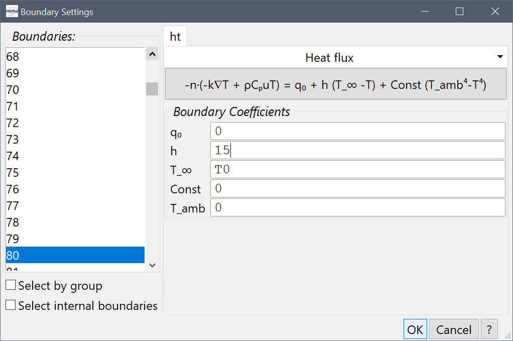
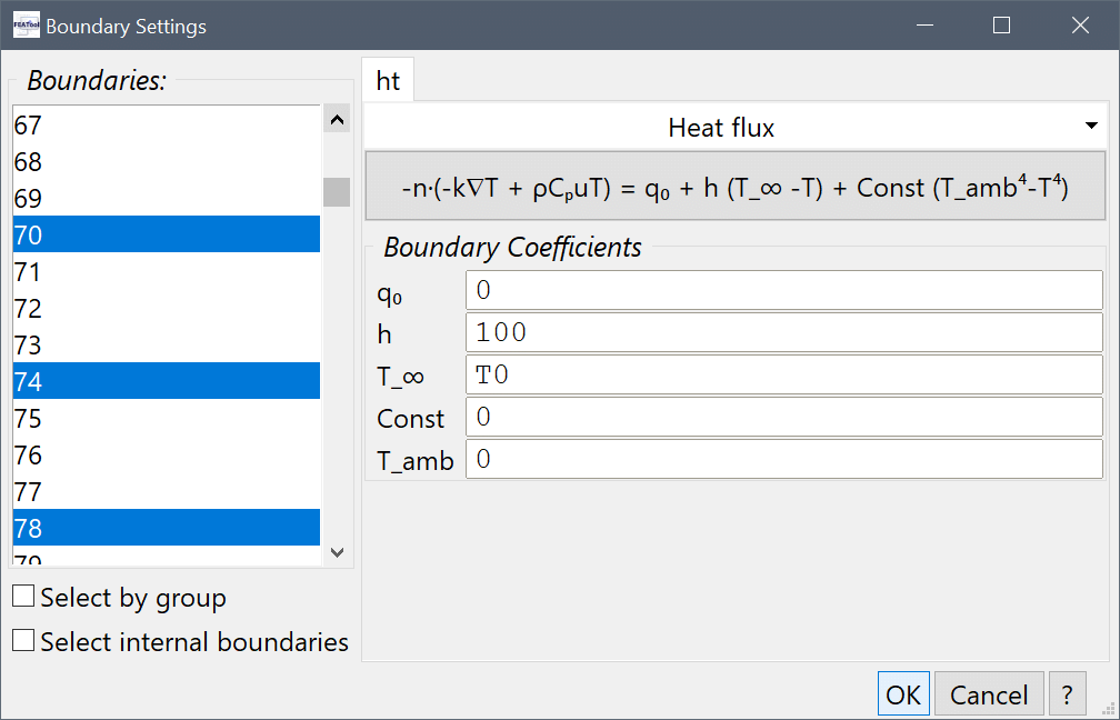
Then select the from and back boundaries (here numbers 4 and 80). and choose the Heat flux from the Heat Transfer drop-down menu.
Enter 15 into the Heat transfer coefficient edit field, and T0 into the Bulk temperature edit field.
Press OK to finish the boundary condition specification.
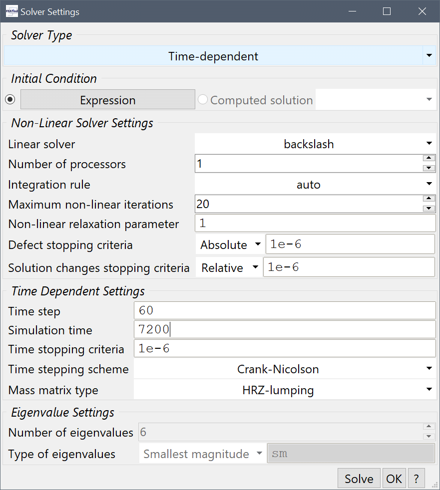
Switch to Solve mode by clicking on the corresponding Mode Toolbar button.
Press the Settings Toolbar button.
Select Time-Dependent from the Solution and solver type drop-down menu, enter 60 into the Time step size edit field, and 7200 into the Duration of time-dependent simulation (maximum time).
Press OK to apply the selected solver settings, and press the = Toolbar button to call the solver. After the problem has been solved the toolbox will automatically switch to postprocessing mode and plot the computed solution.

Now check the temperature in the middle of the failed battery cell (number 10).

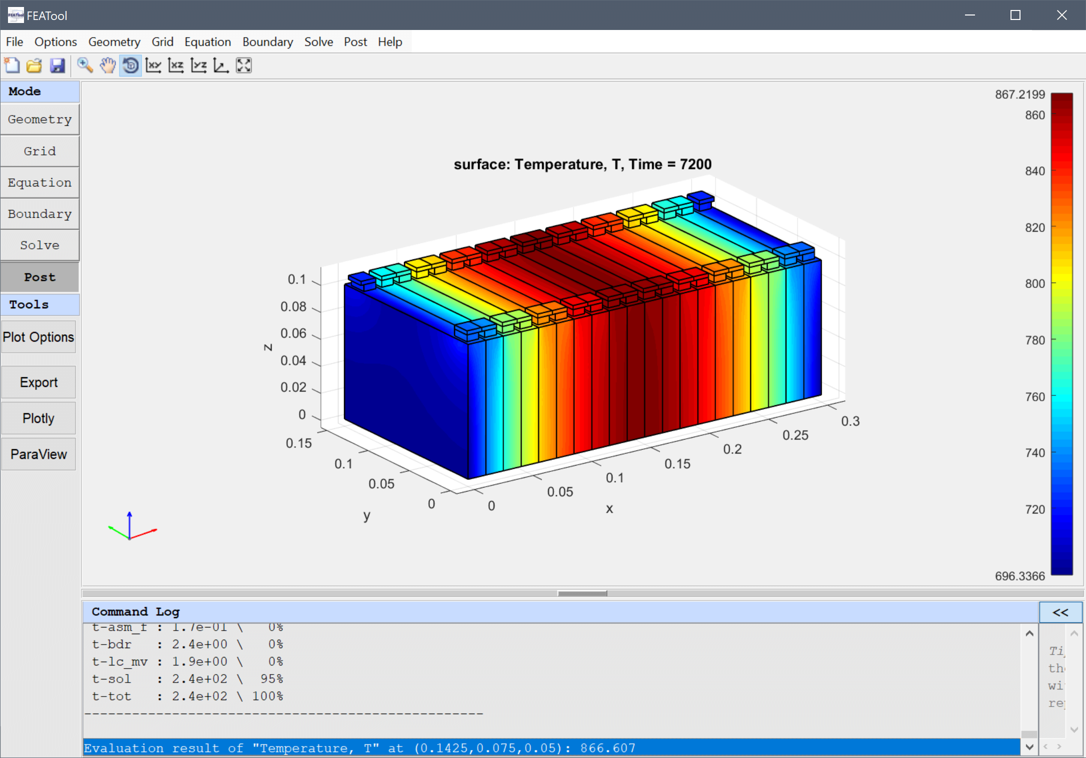
Select Point/Line Evaluation... from the Post menu to open the corresponding dialog box.
Enter 0.1425, 0.075, and 0.05 into the Evaluation coordinates in x, y, and z-direction edit fields, respectively, and press OK.

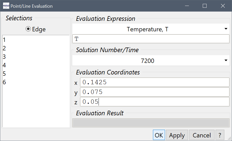
The resulting temperature is printed in the command log. Here it will be around 867 K in the center of the cell which is too high for safety.

We will try to add more cooling to the bottom of the pack, and see how the temperature field changes.

Go back to Boundary mode by clicking on the corresponding Mode Toolbar button.
Select all of the bottom boundaries (here 1, 6, 10, 14, 18, 22, 26, 30, 34, 38, 42, 46, 50, 54, 58, 62, 66, 70, 74, and 78) in the Boundaries list box.
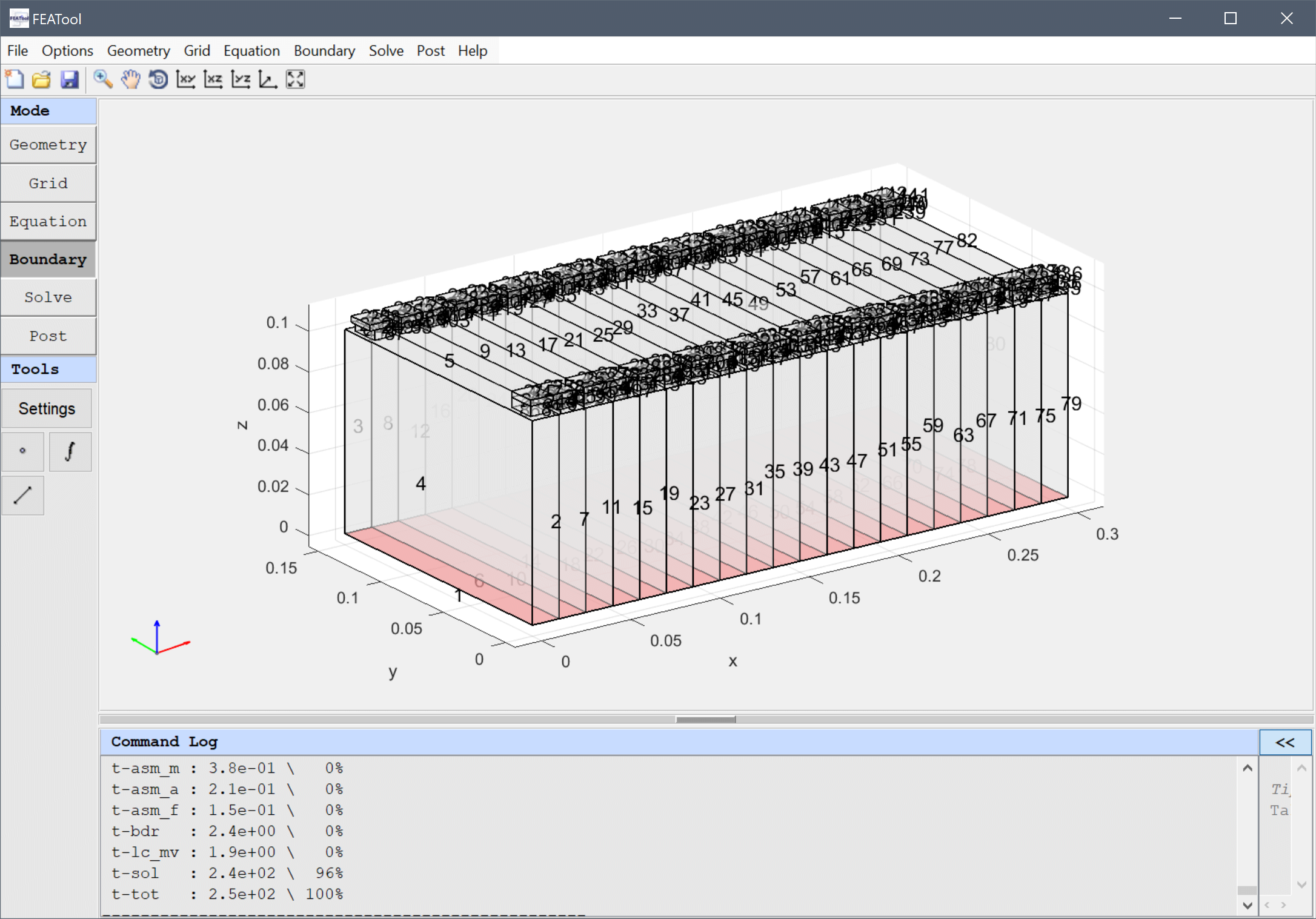
Change to the Heat flux boundary condition, and enter 100 into the Heat transfer coefficient edit field, and T0 into the Bulk temperature edit field.
Press OK to finish the boundary condition specification.
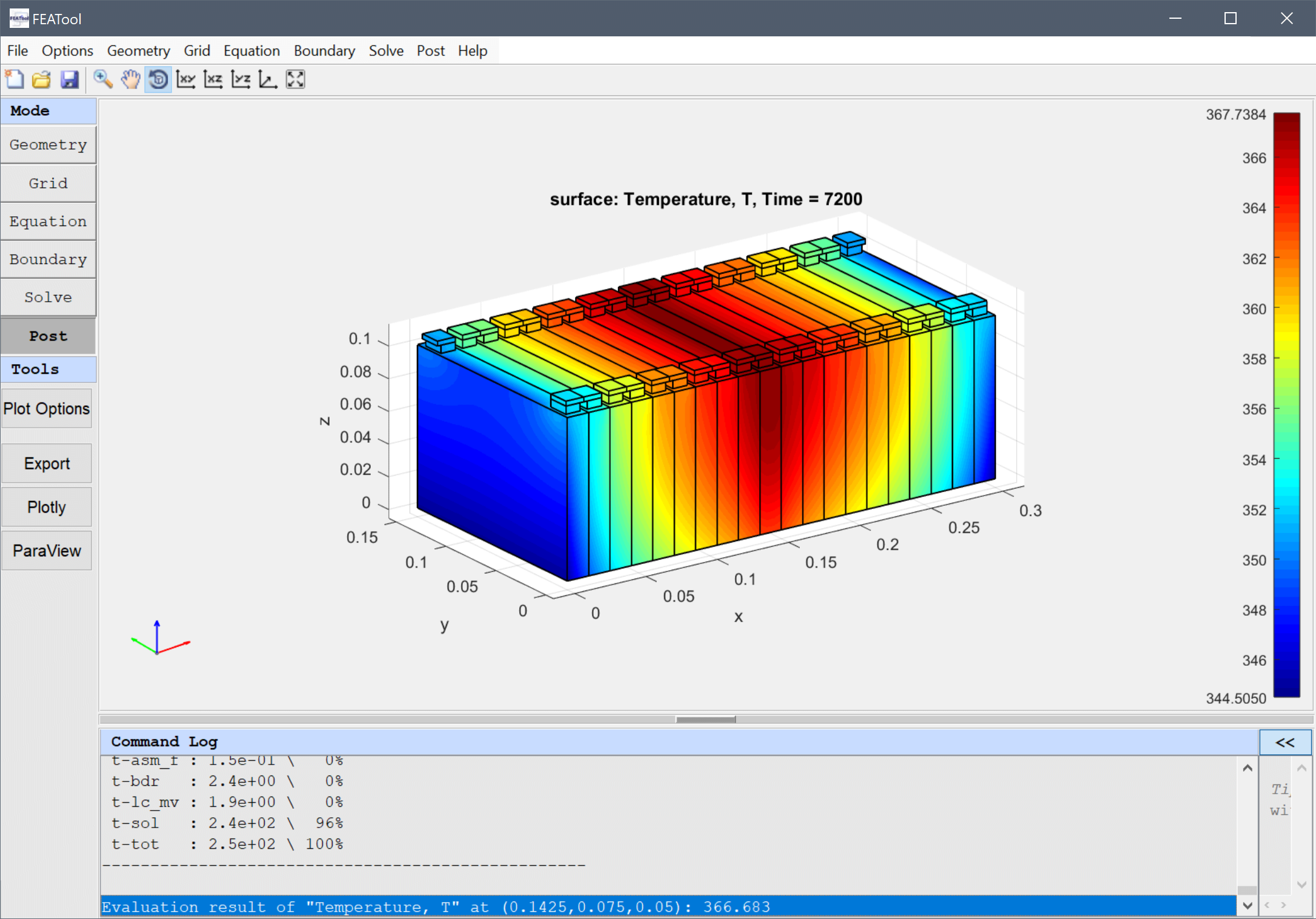
Switch to Solve mode again by clicking on the corresponding Mode Toolbar button.
Press the Restart button, which will use the last solution as initial condition (to save some computational time to reach the final steady state).

After the simulation has finished, we can see that the overall temperature field is much lower now. Again evaluate the temperature in the middle of the failed cell.

Select Point/Line Evaluation... from the Post menu, enter 0.1425, 0.075, and 0.05 into the Evaluation coordinates in x, y, and z-direction edit fields, respectively, and press OK.

The resulting temperature is now much lower, around 367 K, acceptable for our safety and design margins.