Resistive Heating in a Tungsten Filament

This example models resistive Joule heating where the resulting current from an applied electric potential will heat a thin spiral shaped Tungsten wire, such as can be found in incandescent light bulbs. The filament reaches an equilibrium temperature where the internal heat generation is balanced by radiative heat loss through the boundaries.

Two physics modes are involved, conductive media DC for the electric potential V, and heat transfer for the temperature T. Since the coupling is one way where only the heat transfer source term depends on the potential, the model will be solved in two steps. First for the electric potential, and then for the temperature using the pre-calculated potential, this saves computational time.

Tutorial

This model is available as an automated tutorial by selecting Model Examples and Tutorials... > Multiphysics > Resistive Heating in a Tungsten Filament from the File menu. Or alternatively, follow the step-by-step instructions below.

1. To start a new model click the New Model toolbar button, or select New Model... from the File menu.
2. Select the 3D radio button.

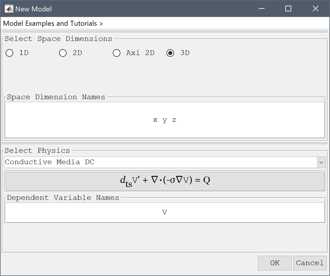
3. Select the Conductive Media DC physics mode from the Select Physics drop-down menu.

   
4. Press OK to finish the physics mode selection.
5. The filament geometry can be generated by creating a circle in a workplane and revolving it. To define the workplane select 2D Workplane... from the Geometry menu.

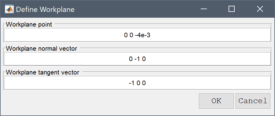
6. Set the Workplane normal vector to 0 -1 0 and Workplane tangent vector to -1 0 0 in the dialog box. The tangent will represent the x-axis in the local 2D workplane coordinate system, while the cross product of the normal and tangent will represent the local y-axis. If one looks at the 3D view a preview of the local axis can be seen with the normal in blue, x-axis red, and y-axis yellow orthogonal vectors.

   
7. Press OK to create the workplane. This will open a new 2D GUI for planar geometry definition on the local workplane.

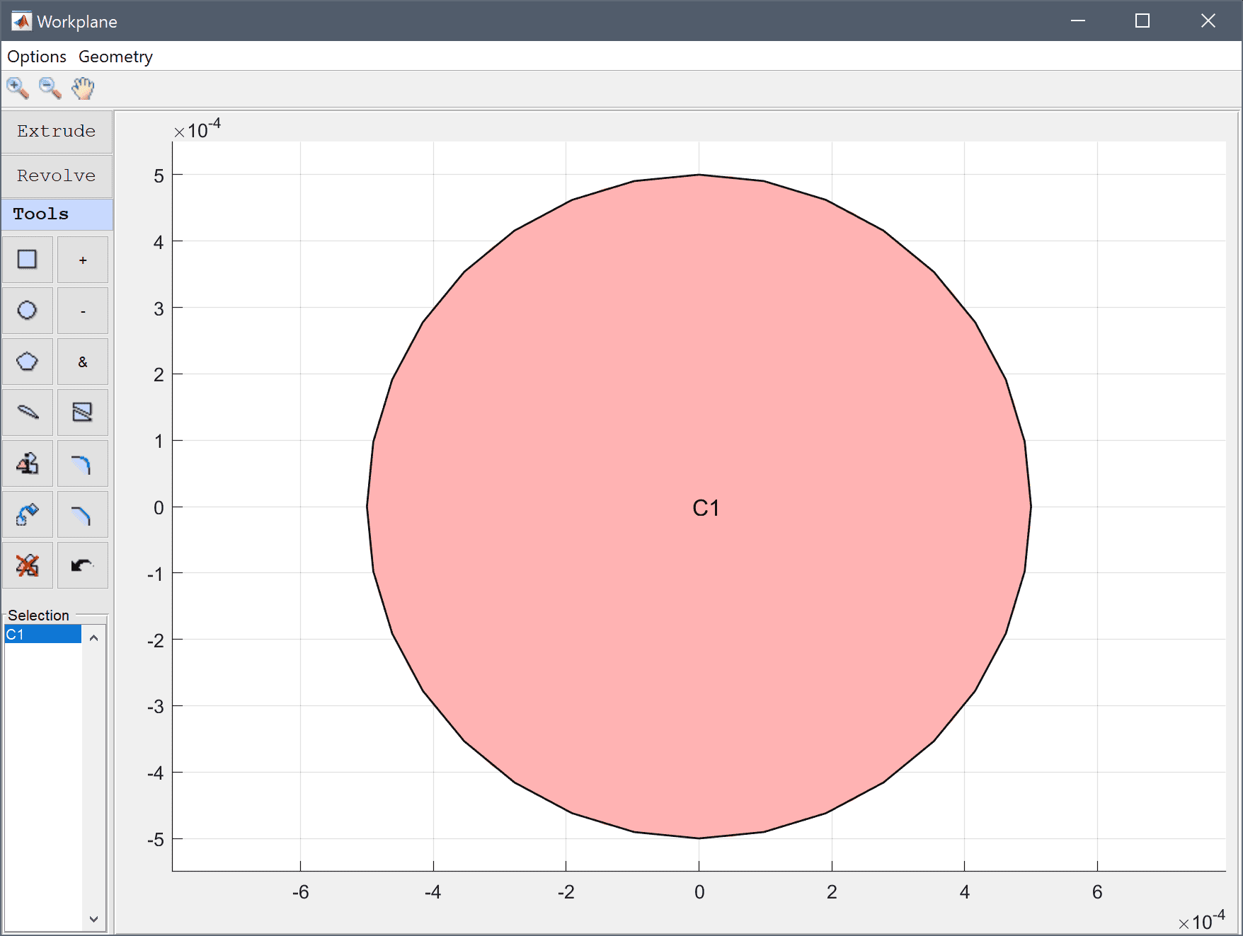
Create a circle at the origin with radius 5e-4.

1. Select Circle from the Geometry menu.
2. Enter 5e-4 into the radius edit field.

3. Press OK to finish and close the dialog box.

   
4. Select the circle C1 in the geometry object Selection list box and press the Revolve button.

The circle should be rotated 3 full revolutions (1080 degrees) with a pitch of 1.8e-3 around the vector (1 0 0) with base at (0 -4e-3 0).

1. Enter 1.8e-3 into the Revolution pitch (axial offset distance per full revolution) edit field.
2. Enter 1080 into the Revolution angle edit field.
3. Enter 0 -4e-3 0 into the Revolution axis reference point edit field.

4. Enter 1 0 0 into the Revolution axis vector edit field.

   

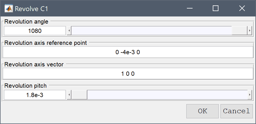
Press OK to create the revolved geometry object, and then close the 2D Workplane GUI to return control to the 3D view.

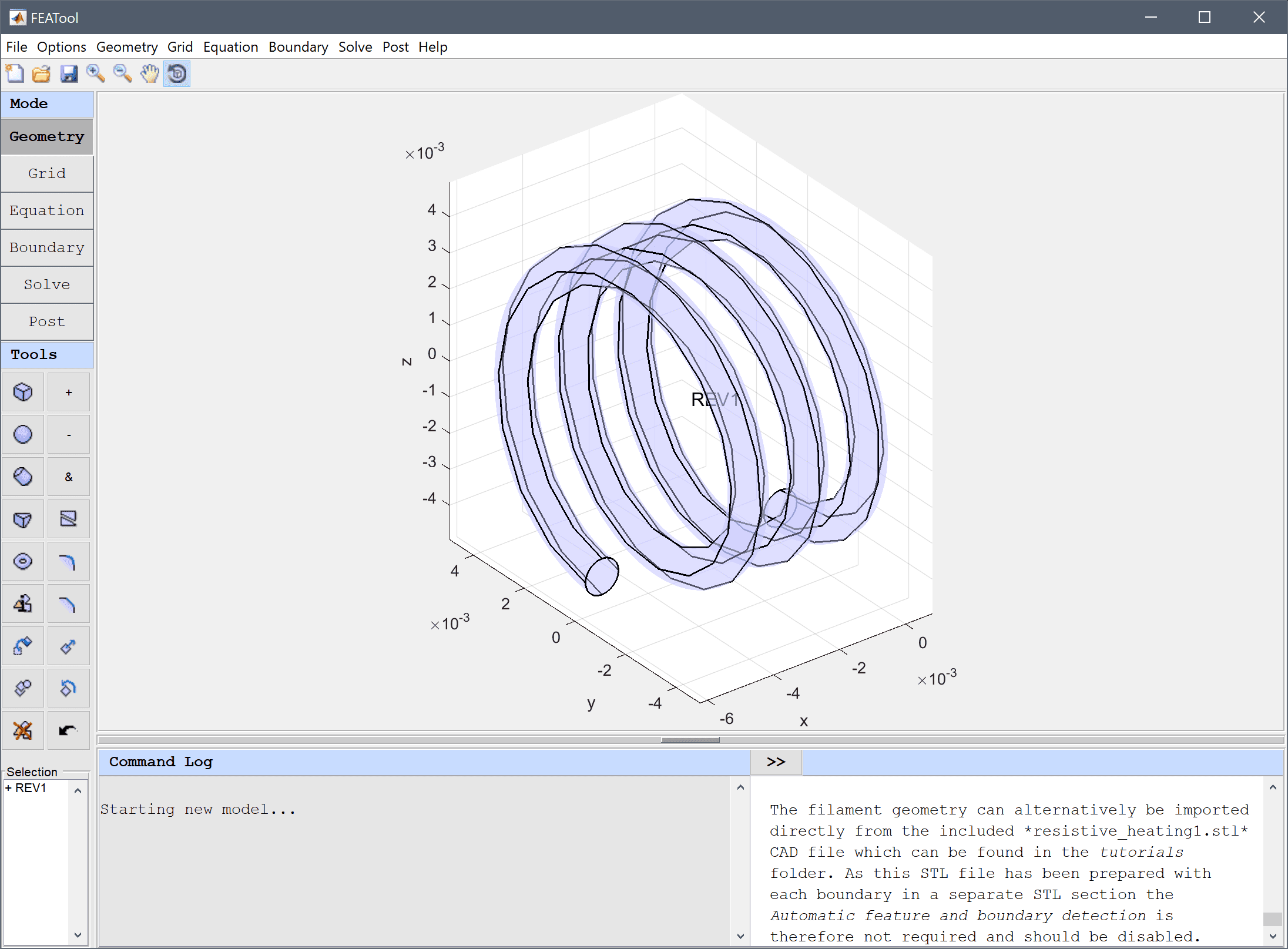
The filament geometry can alternatively be imported directly from the included resistive_heating1.stl CAD file which can be found in the tutorials folder. As this STL file has been prepared with each boundary in a separate STL section the Automatic feature and boundary detection is therefore not required and should be disabled.

1. Switch to Grid mode by clicking on the corresponding Mode Toolbar button.
2. Press the Settings Toolbar button.
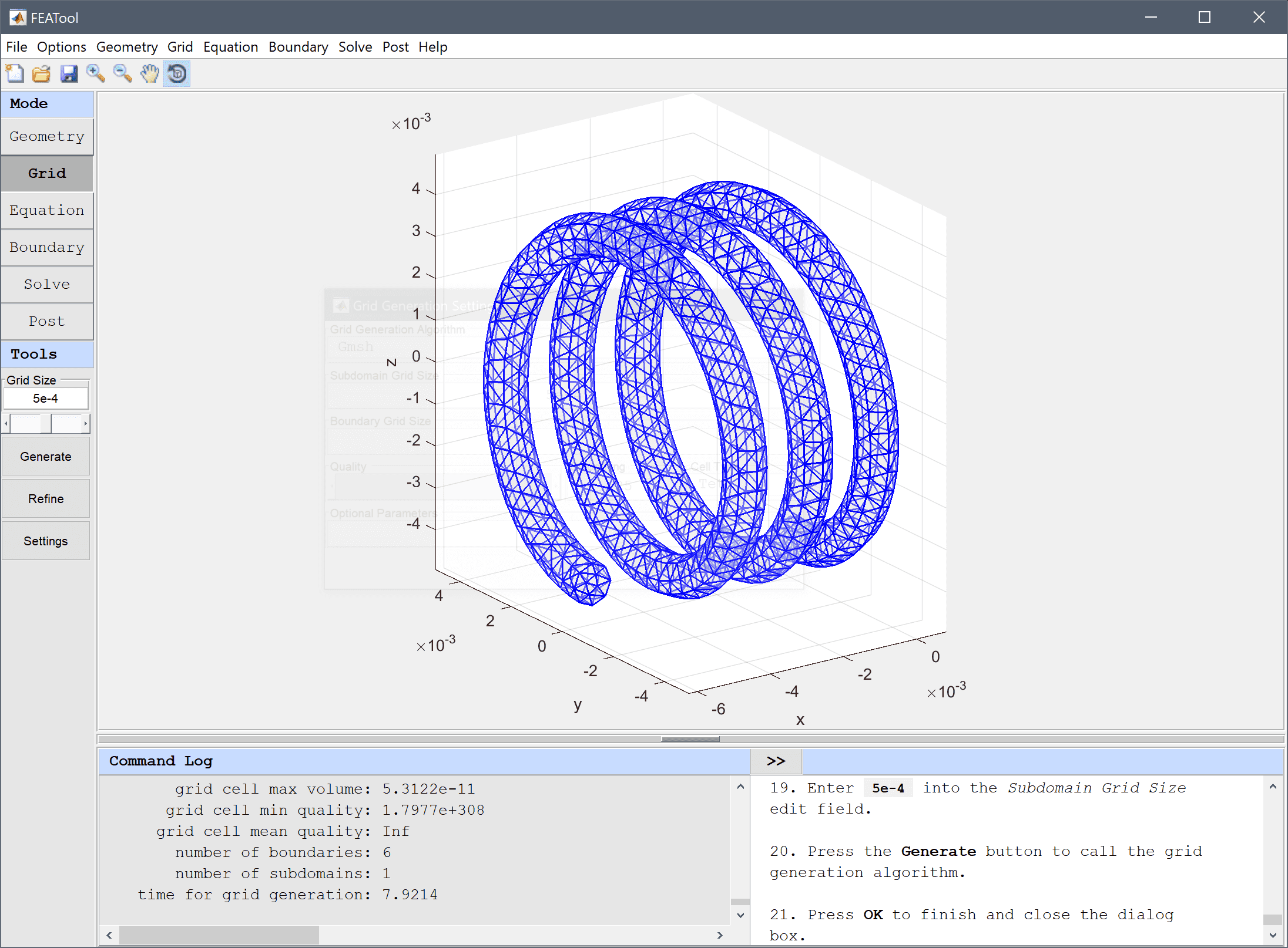
3. Enter 5e-4 into the Subdomain Grid Size edit field.

4. Press the Generate button to call the grid generation algorithm.

   

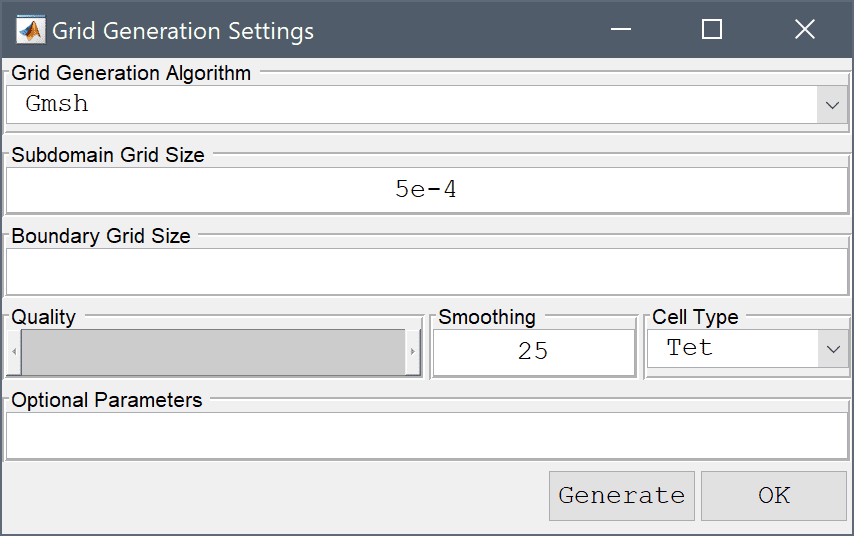
5. Press OK to finish and close the dialog box.

   
6. Switch to Equation mode by clicking on the corresponding Mode Toolbar button.

7. Enter 1/52.8e-9 into the Electric conductivity edit field.

   
8. Switch to the + tab.
9. Select the Heat Transfer physics mode from the Select Physics drop-down menu.
10. Press the Add Physics >>> button.
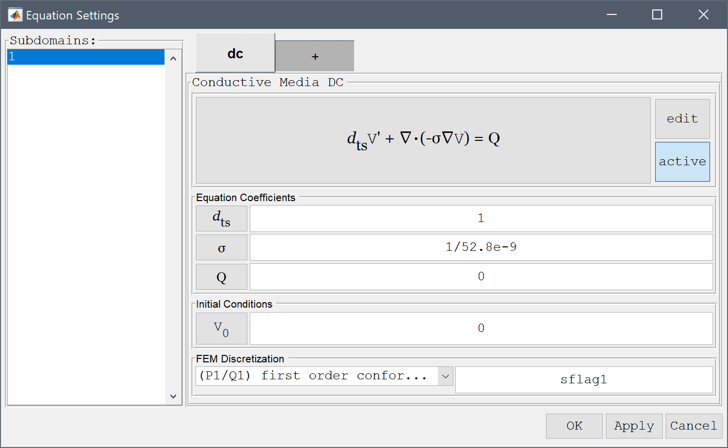
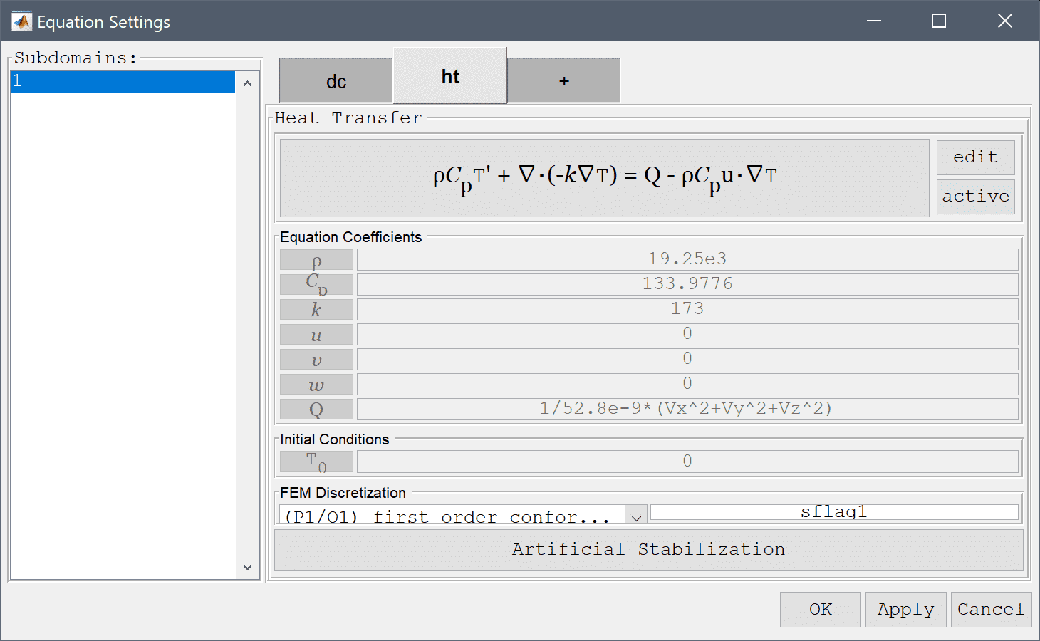
11. Enter 19.25e3 into the Density edit field.
12. Enter 133.9776 into the Heat capacity edit field.
13. Enter 173 into the Thermal conductivity edit field.
14. Enter the expression 1/52.8e-9*(Vx^2+Vy^2+Vz^2) for the temperature source term, effectively coupling the gradient of the electric potential to the temperature field.

15. In the first step, only the potential V will be solved for, so deactivate the temperature by clicking on the Active button. This will deactivate a selected physics mode in the specific subdomains, or here deactivate it completely.

    
16. Press OK to finish the equation and subdomain settings specification.
17. Switch to Boundary mode by clicking on the corresponding Mode Toolbar button.

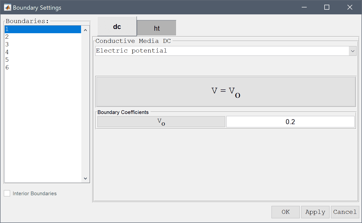
Apply a potential difference of 0.2 V between the two ends.

1. Select 1 and 6 in the Boundaries list box.
2. Select Electric potential from the Conductive Media DC drop-down menu.
3. Enter 0 into the Electric potential edit field.
4. Select 1 in the Boundaries list box.

5. Enter 0.2 into the Electric potential edit field.

   
6. Switch to the ht tab.
7. To specify the radiative boundary condition, select Heat flux for all but the end boundaries and enter the coefficient for the radiative Constant and surrounding ambient temperature Tamb.
8. Enter 5.670367e-8 into the Radiation constant edit field.

9. Enter 80+273.15 into the Ambient temperature edit field.

   

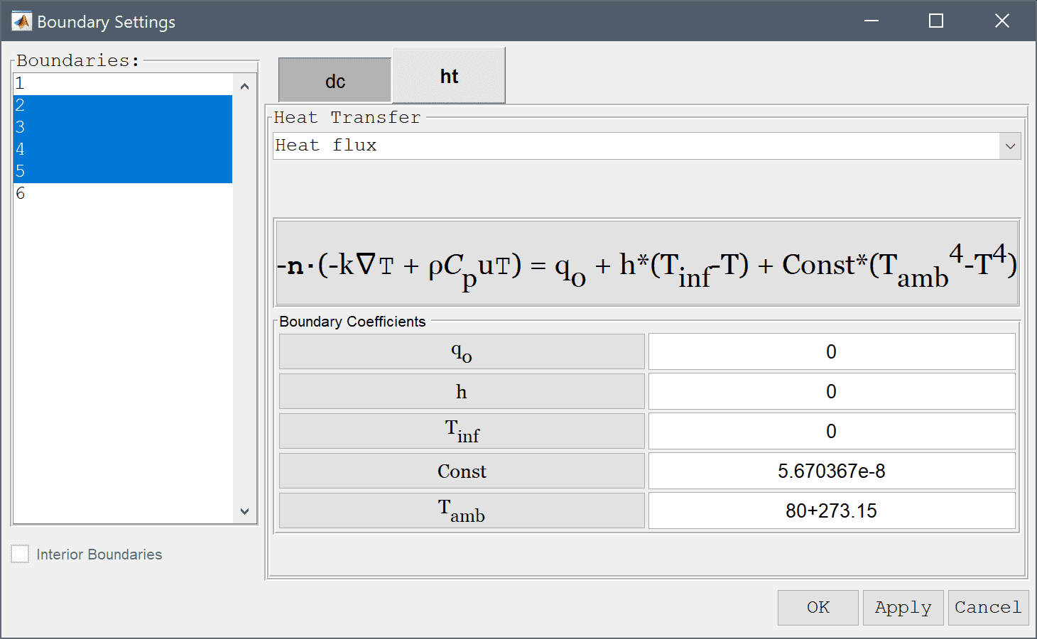
The end boundaries are assumed held at room temperature.

1. Select 1 and 6 in the Boundaries list box.
2. Select Temperature from the Heat Transfer drop-down menu.
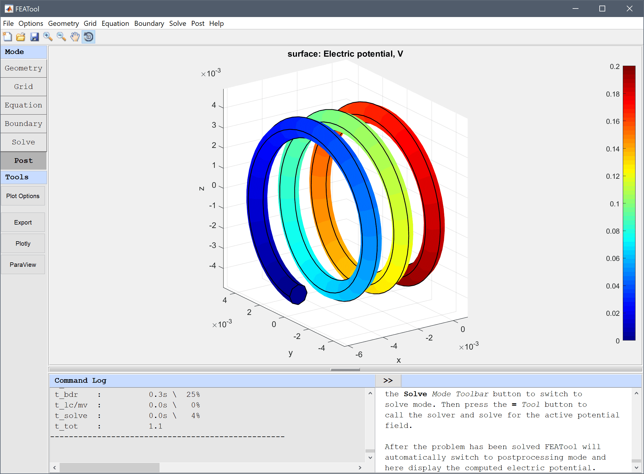
3. Enter 20+273.15 into the Temperature edit field.
4. Press OK to finish the boundary condition specification.
5. Now that the problem is fully specified, press the Solve Mode Toolbar button to switch to solve mode. Then press the = Tool button to call the solver and solve for the active potential field.

After the problem has been solved FEATool will automatically switch to postprocessing mode and here display the computed electric potential.

To solve for the temperature field, switch back to Equation mode activate the heat transfer physics mode and deactivate the electric potential.

1. Press the active toggle button.
2. Switch to the ht tab.
3. Press the active toggle button.
4. Press OK to finish the equation and subdomain settings specification.
5. Switch to Solve mode by clicking on the corresponding Mode Toolbar button.

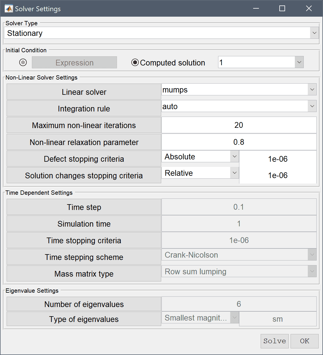
The current solution has to be used as initial guess to use the computed potential since it is deactivated, also decrease the Non-linear relaxation parameter to help with convergence.

1. Press the Settings Toolbar button.
2. Select the Computed solution radio button.

3. Enter 0.8 into the Non-linear relaxation parameter (ratio of new to old solution to use) edit field.

   
4. Press the Solve button.

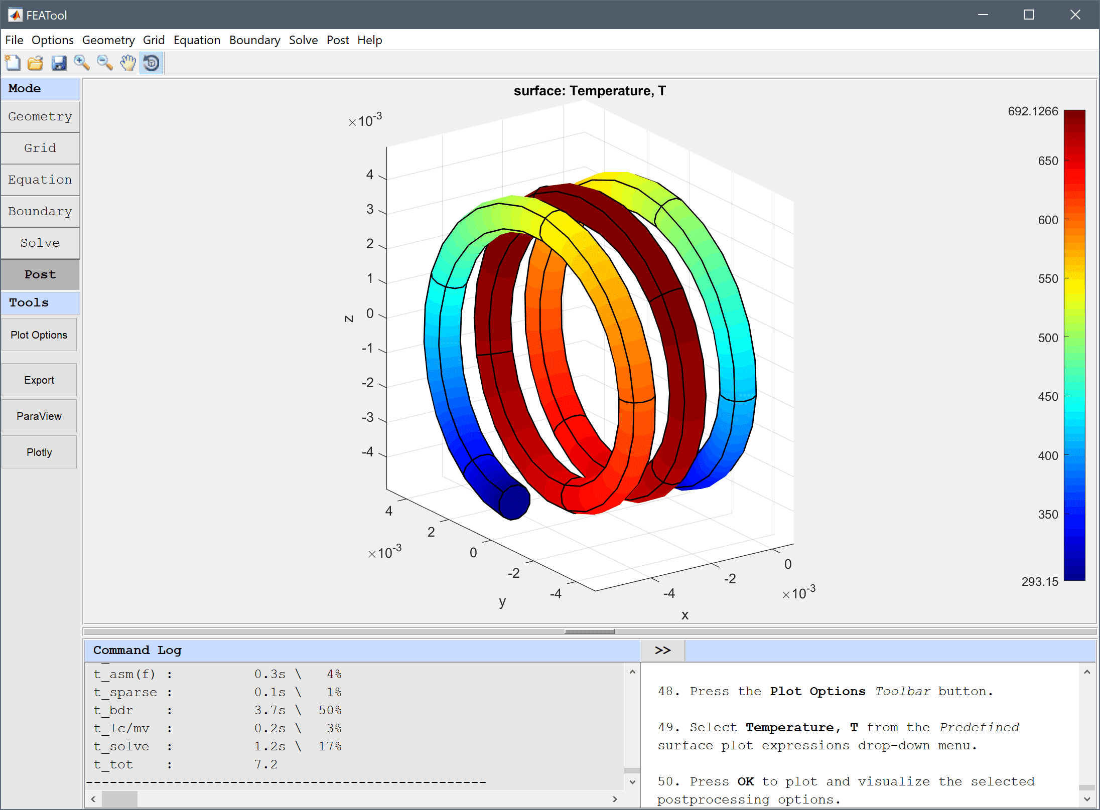
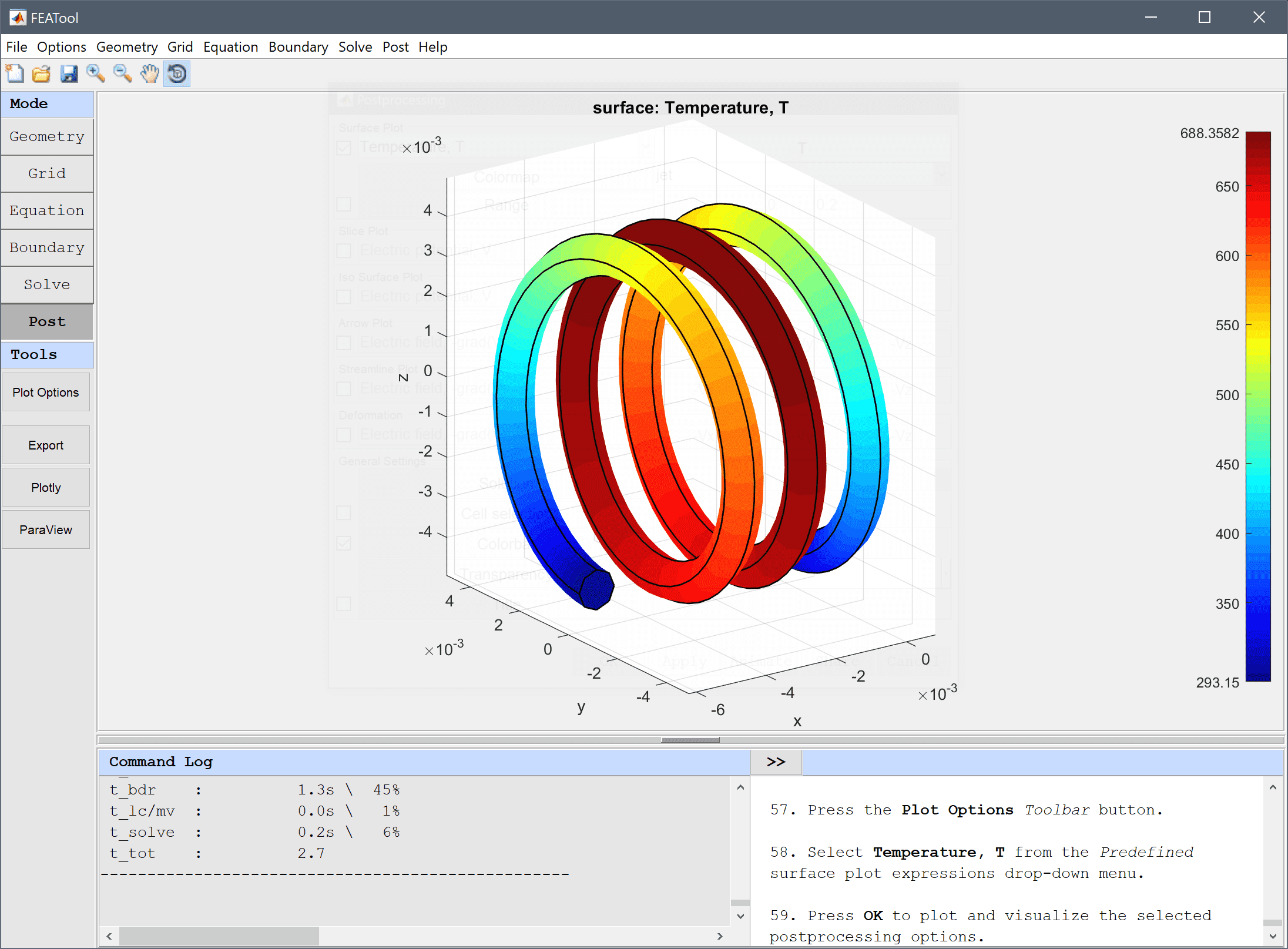
After the solver has converged, plot the temperature and verify that the maximum temperature is around 690.

1. Press the Plot Options Toolbar button.
2. Select Temperature, T from the Predefined surface plot expressions drop-down menu.

3. Press OK to plot and visualize the selected postprocessing options.

   

The resistive heating in a tungsten filament multiphysics model has now been completed and can be saved as a binary (.fea) model file, or exported as a programmable MATLAB m-script text file (available as the example ex_resistive_heating1 script file), or GUI script (.fes) file.