Flow in Porous Media

Axisymmetric laminar fluid flow in a diffusor duct or reaction chamber blocked by sections of a porous material. The model features several partially active subdomains with the Brinkman equations governing the fluid flow. The flow field with and without the porous material is compared.

Tutorial

This model is available as an automated tutorial by selecting Model Examples and Tutorials... > Multiphysics > Flow in Porous Media from the File menu. Or alternatively, follow the step-by-step instructions below.

1. To start a new model click the New Model toolbar button, or select New Model... from the File menu.
2. Select the Axisymmetry radio button.

First is to solve a pure laminar flow problem without the porous domains.

1. Select the Navier-Stokes Equations physics mode from the Select Physics drop-down menu.
2. Press OK to finish the physics mode selection.
3. Select Polygon from the Geometry menu.

Enter the following data into the Point coordinates table.

	r	z
1	0	0
2	0.002	0
3	0.005	0.003
4	0.005	0.01
5	0.002	0.013
6	0	0.013

1. Press OK to finish and close the dialog box.
2. Select Rectangle from the Geometry menu.
3. Enter 4e-3 into the y_min edit field.
4. Enter 8e-3 into the y_max edit field.
5. Enter 1e-3 into the x_max edit field.
6. Press OK to finish and close the dialog box.
7. Select Rectangle from the Geometry menu.
8. Enter 1.5e-3 into the x_min edit field.
9. Enter 3.5e-3 into the x_max edit field.
10. Enter 4e-3 into the y_min edit field.
11. Enter 8e-3 into the y_max edit field.
12. Press OK to finish and close the dialog box.
13. Select R1 in the geometry object Selection list box.
14. Press the Copy and/or transform selected geometry object Toolbar button.
15. Select the Make copy of geometry object check box.
16. Enter 4e-3 0 into the Space separated string of displacement lengths edit field.
17. Press OK to finish and close the dialog box.
18. Switch to Grid mode by clicking on the corresponding Mode Toolbar button.
19. Press the Settings Toolbar button.

Specific grid sizes for subdomains and boundaries can be prescribed directly in the Grid Settings dialog box. Here the grid size in the outer domain is set to three times the porous domains.

1. Enter 1.5e-4*[3 1 1 1] into the Subdomain Grid Size edit field.
2. Press the Generate button to call the grid generation algorithm.
3. Press OK to finish and close the dialog box.
4. Switch to Equation mode by clicking on the corresponding Mode Toolbar button.
5. Select all subdomains 1-4 in the Subdomains list box.
6. Enter 1.2 into the Density edit field.
7. Enter 1.8e-5 into the Viscosity edit field.
8. Press OK to finish the equation and subdomain settings specification.
9. Switch to Boundary mode by clicking on the corresponding Mode Toolbar button.
10. Select 1 in the Boundaries list box.
11. Select Inlet/velocity from the Navier-Stokes Equations drop-down menu.
12. Enter 2e-2 into the Velocity in z-direction edit field.
13. Select 6 in the Boundaries list box.
14. Select Outflow/pressure from the Navier-Stokes Equations drop-down menu.
15. Select 7-9 in the Boundaries list box.
16. Select Symmetry/slip from the Navier-Stokes Equations drop-down menu.
17. Press OK to finish the boundary condition specification.
18. Switch to Solve mode by clicking on the corresponding Mode Toolbar button.
19. Press the = Toolbar button to call the solver. After the problem has been solved FEATool will automatically switch to postprocessing mode and plot the computed solution.
20. Press the Plot Options Toolbar button.
21. Select the Contour Plot check box.
22. Select Pressure from the Predefined contour plot expressions drop-down menu.
23. Select the Arrow Plot check box.
24. Press OK to plot and visualize the selected postprocessing options.

By plotting the Velocity field at the mid point one can see that the flow decreases smoothly towards the edges.

1. Select Point/Line Evaluation... from the Post menu.
2. Select Velocity field from the Evaluation Expression drop-down menu.
3. Enter 0:0.005/100:0.005 into the Evaluation coordinates in r-direction edit field.
4. Enter 0.006 into the Evaluation coordinates in z-direction edit field.
5. Press OK to finish and close the dialog box.

Now go back to Equation mode and add the Brinkman Equations physics mode which will account for the porous domains.

1. Switch to Equation mode by clicking on the corresponding Mode Toolbar button.
2. Switch to the + tab.
3. Select the Brinkman Equations physics mode from the Select Physics drop-down menu.
4. Press the Add Physics >>> button.
5. Select 2-4 in the Subdomains list box.
6. Enter 1.2 into the Density edit field.
7. Enter 1.8e-5 into the Viscosity edit field.
8. Enter 2e-7 into the Permeability edit field.

Deactivate the Brinkman Equations physics mode in the outer domain.

1. Select 1 in the Subdomains list box.
2. Press the active toggle button.

Similarly, deactivate the Navier-Stokes Equations physics mode in the inner porous domains.

1. Switch to the ns tab.
2. Select 2-4 in the Subdomains list box.
3. Press the active toggle button.
4. Press OK to finish the equation and subdomain settings specification.
5. Switch to Boundary mode by clicking on the corresponding Mode Toolbar button.

The two physics modes are coupled via setting the corresponding velocities equal at the shared boundaries.

1. Select 11-20 in the Boundaries list box.
2. Select Inlet/velocity from the Navier-Stokes Equations drop-down menu.
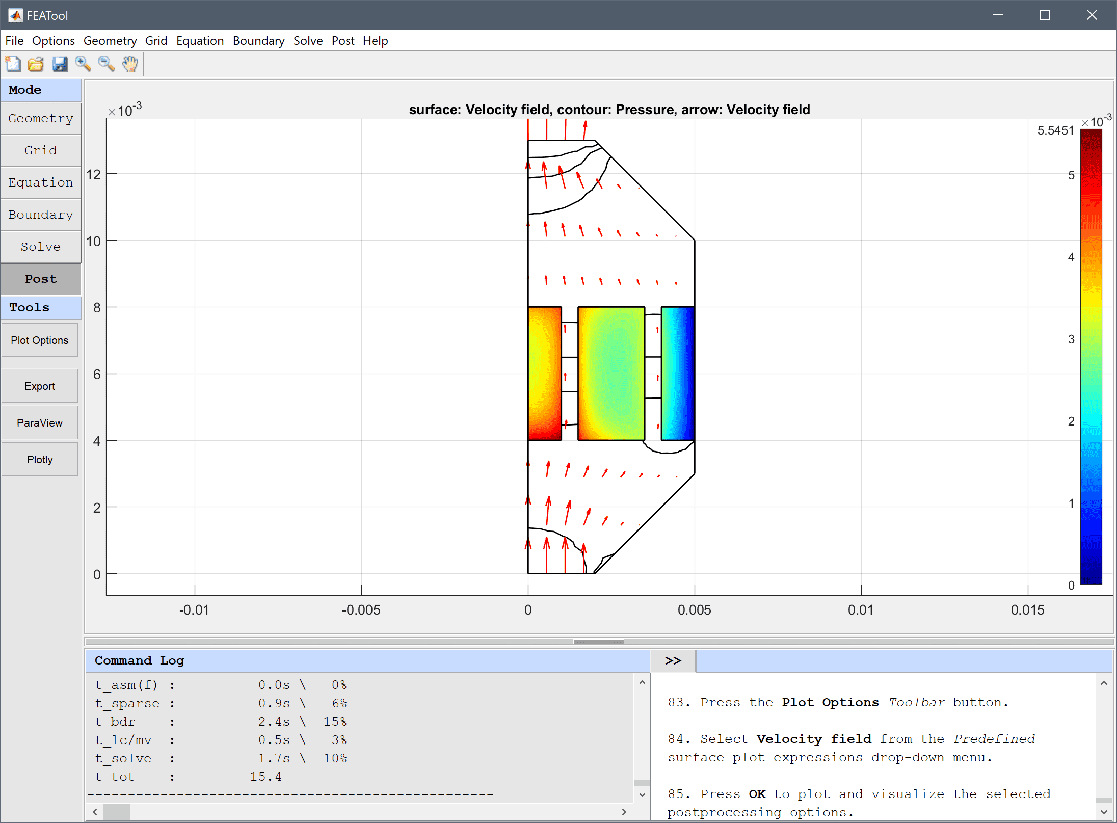
3. Enter u2 into the Velocity in r-direction edit field.
4. Enter w2 into the Velocity in z-direction edit field.
5. Switch to the br tab.
6. Select Inlet/velocity from the Brinkman Equations drop-down menu.
7. Enter u into the Velocity in r-direction edit field.
8. Enter w into the Velocity in z-direction edit field.
9. Select 9 in the Boundaries list box.
10. Select Symmetry/slip from the Brinkman Equations drop-down menu.
11. Press OK to finish the boundary condition specification.
12. Switch to Solve mode by clicking on the corresponding Mode Toolbar button.
13. Press the = Toolbar button to call the solver. After the problem has been solved FEATool will automatically switch to postprocessing mode and plot the computed solution.

There now exists two sets of postprocessing variables, one for each physics mode. Plot and compare the magnitude of the Velocity field for both the porous and outer domains.

1. Press the Plot Options Toolbar button.
2. Select Velocity field from the Predefined surface plot expressions drop-down menu.
3. Press OK to plot and visualize the selected postprocessing options.

Also again plot magnitude of the Velocity field at the mid point line. As nan values are returned for queries outside the valid domain, one can use the setnan function to plot both curves together.

1. Select Point/Line Evaluation... from the Post menu.
2. Enter setnan(sqrt(u^2+w^2),0) + setnan(sqrt(u2^2+w2^2),0) into the edit field.
3. Enter 0:0.005/100:0.005 into the Evaluation coordinates in r-direction edit field.
4. Enter 0.006 into the Evaluation coordinates in z-direction edit field.
5. Press OK to finish and close the dialog box.

Compared to the smooth flow before, the flow now is irregular with two peaks between the porous domains.

The flow in porous media multiphysics model has now been completed and can be saved as a binary (.fea) model file, or exported as a programmable MATLAB m-script text file, or GUI script (.fes) file.

CLI Postprocessing

To visualize the full 3D solution from the axisymmetic model, the data can be exported and processed on the MATLAB command line interface (CLI) console with the Export Model Data Struct to MATLAB option from the File menu. The postrevolve and postplot functions can then be applied to revolve and visualize the data, for example

fea_revolved = postrevolve( fea, 24, 0.75 );

postplot( fea_revolved, 'surfexpr', 'setnan(sqrt(u^2+w^2)) + setnan(p2*1e1)', ...
          'parent', figure, 'axis', 'off', 'colorbar', 'off' )
view(60, 30)