Heat Induced Stress in a Brake Disc

This multiphysics model examines temperature and heat induced stresses for one braking cycle in a brake disc assembly, and involves coupling of the stress-strain and heat transfer physics modes. The braking process consists of applying a brake pad to the front part of the disc which induces heat through friction, and results in build up of stresses and strains in the brake disc. Both rotational and axial symmetry is used to reduce the computational cost. Simulations have been performed with the geometry and material parameters given in the reference [1] resulting in the final temperature and stress fields shown in the following figures.

The resulting temperature and stress curves on the disk surface at various times agree well with the results computed with the Nastran FEA software [1].

Tutorial

This model is available as an automated tutorial by selecting Model Examples and Tutorials... > Multiphysics > Heat Induced Stress in a Brake Disc from the File menu.

1. To start a new model click the New Model toolbar button, or select New Model... from the File menu.
2. Select the Axisymmetry radio button.
3. Select the Axisymmetric Stress-Strain physics mode from the Select Physics drop-down menu.
4. Press OK to finish the physics mode selection.

The geometry only includes the cross section of the brake disc, and not the brake pad. Although this could be modeled with a single rectangle, the brake pad only touches part of the disc, so two rectangles are used to split the boundary into sections.

1. Select Rectangle from the Geometry menu.
2. Enter 66e-3 into the x_min edit field.
3. Enter 75.5e-3 into the x_max edit field.
4. Enter 5.5e-3 into the y_max edit field.
5. Press OK to finish and close the dialog box.
6. Select Rectangle from the Geometry menu.
7. Enter 75.5e-3 into the x_min edit field.
8. Enter 113.5e-3 into the x_max edit field.
9. Enter 5.5e-3 into the y_max edit field.
10. Press OK to finish and close the dialog box.
11. Switch to Grid mode by clicking on the corresponding Mode Toolbar button.
12. Enter 0.0005 into the Grid Size edit field.
13. Press the Generate button to call the grid generation algorithm.
14. Switch to Equation mode by clicking on the corresponding Mode Toolbar button.

The material parameters are taken from the reference assuming the brake disc is made of cast iron. Make sure that the material parameters are specified in both subdomain halves of the disc.

1. Select 1 and 2 in the Subdomains list box.
2. Enter 0.29 into the Poisson's ratio edit field.
3. Enter 99.97e9 into the Modulus of elasticity edit field.
4. Enter 7100 into the Density edit field.
5. Enter 1.08e-5 into the Thermal expansion coefficient edit field.
6. Enter T-(20+273.15) into the Temperature edit field.
7. Switch to the + tab.
8. Select the Heat Transfer physics mode from the Select Physics drop-down menu.
9. Press the Add Physics >>> button.
10. Enter 7100 into the Density edit field.
11. Enter 51/1.44e-5/7100 into the Heat capacity edit field.
12. Enter 51 into the Thermal conductivity edit field.
13. Press OK to finish the equation and subdomain settings specification.
14. Switch to Boundary mode by clicking on the corresponding Mode Toolbar button.

Symmetry with zero normal displacement is assumed at the lower z = 0 boundaries.

1. Select 1 and 4 in the Boundaries list box.
2. Select the Fixed displacement, w radio button.
3. Switch to the ht tab.

The brake force is applied to the upper right section of the disc which magnitude is calculated as a function of the material of the disc and pad with a friction factor. See the reference for more details.

1. Select 6 in the Boundaries list box.
2. Select Heat flux from the Heat Transfer drop-down menu.
3. Enter 7109581.6204*r*(1-t/3.96) into the Inward heat flux edit field.
4. Press OK to finish the boundary condition specification.
5. Switch to Solve mode by clicking on the corresponding Mode Toolbar button.
6. Press the Settings Toolbar button.

Select Time-Dependent analysis with a simulation time of 3.96 seconds, and also set the initial temperature to 20 °C.

1. Select Time-Dependent from the Solution and solver type drop-down menu.
2. Press the Expression button.
3. Enter 20+273.15 into the Initial condition for T in subdomain 1 edit field.
4. Enter 20+273.15 into the Initial condition for T in subdomain 2 edit field.
5. Press OK to finish and close the dialog box.
6. Enter 3.96 into the Duration of time-dependent simulation (maximum time) edit field.
7. Enter 3.96/50 into the Time step size edit field.
8. Press the Solve button.

After the simulation has completed, inspect the stress and temperature distributions at different times. Especially for the early times it is very clear that both the temperature and stress are located at the interface between disc and pad, and later spreads throughout the disc.

1. Press the Plot Options Toolbar button.
2. Select the Contour Plot check box.
3. Press Apply to plot and visualize the selected postprocessing options.
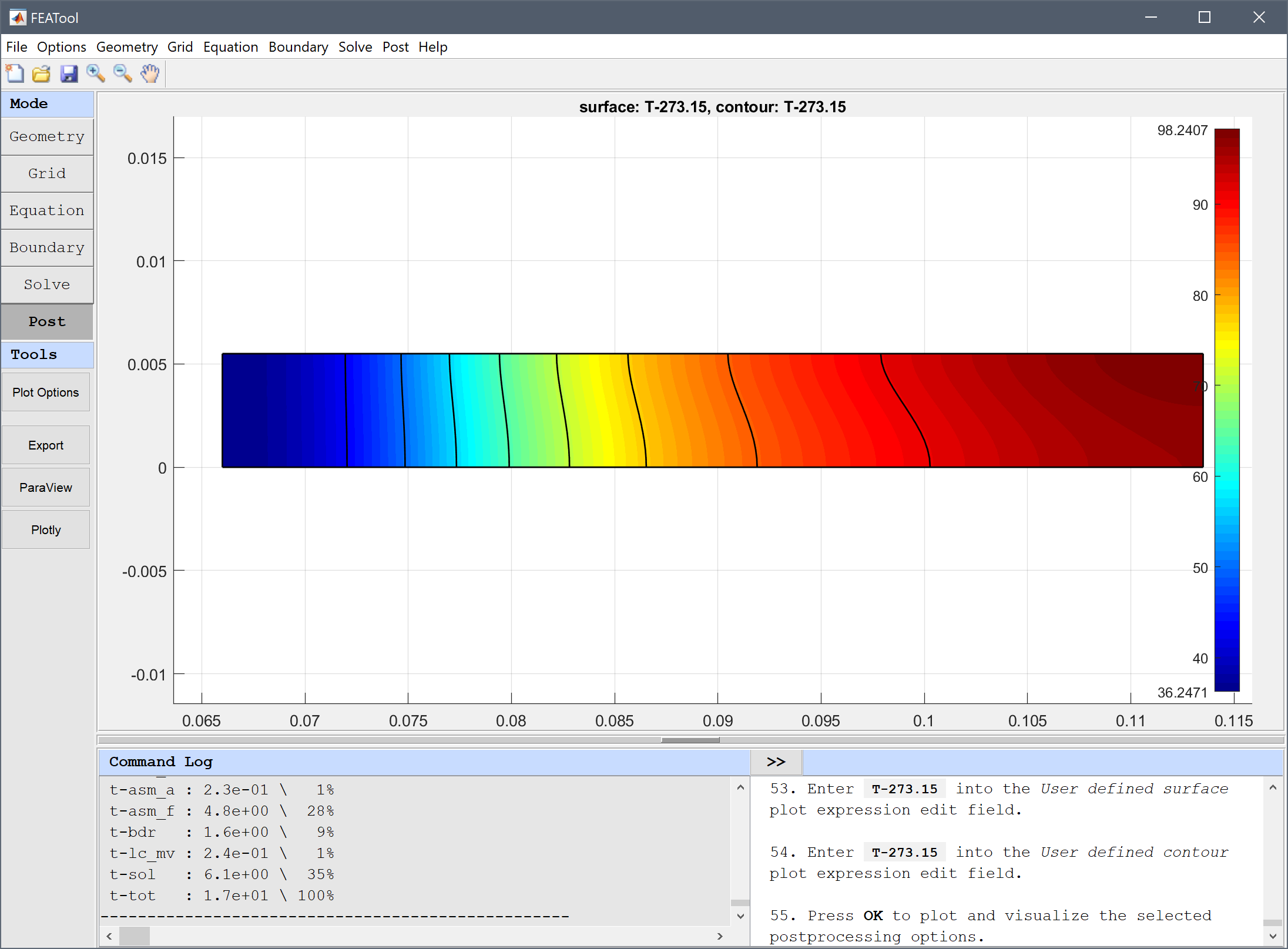
4. Enter T-273.15 into the User defined surface plot expression edit field.
5. Enter T-273.15 into the User defined contour plot expression edit field.
6. Press OK to plot and visualize the selected postprocessing options.

The temperature has increased significantly at the final time, and should span between about 35 and 90 degrees.

The heat induced stress in a brake disc multiphysics model has now been completed and can be saved as a binary (.fea) model file, or exported as a programmable MATLAB m-script text file (available as the example ex_axistressstrain4 script file), or GUI script (.fes) file.

Reference

[1] Adamowicz A. Axisymmetric FE Model to Analysis of Thermal Stresses in a Brake Disk. Journal of Theoretical and Applied Mechanics, 53, 2, pp. 357-370, Warsaw, 2015.