|
|
FEATool Multiphysics
v1.18.0
Finite Element Analysis Toolbox
|
|
|
FEATool Multiphysics
v1.18.0
Finite Element Analysis Toolbox
|
This multiphysics model illustrates natural convection effects in a unit square domain using the Boussinesq approximation. The model involves a Navier-Stokes equations physics mode, representing the fluid flow with solid wall or no-slip boundary conditions everywhere. In addition a heat transfer physics mode is added to model the temperature field. The top and bottom boundaries are perfectly insulated while the left boundary is prescribed a temperature of 1 and the right zero.
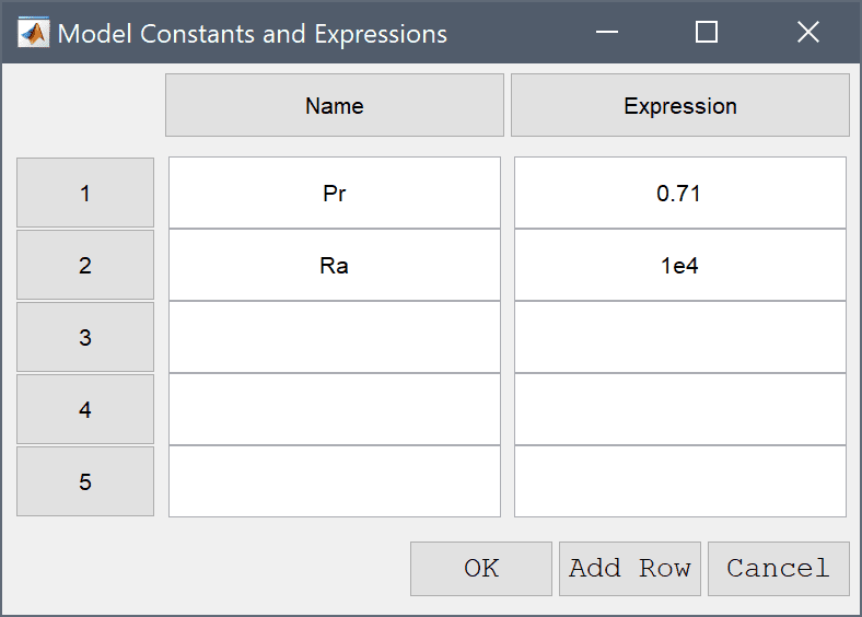
The physics modes are two way coupled through the vertical source term in the Navier-Stokes equations, Pr·Ra·T, and the velocities transporting the temperature coming directly from the fluid flow. First, the Prandtl and Rayleigh numbers are set to Pr = 0.71 and Ra = 103, respectively, after which the Ra number will be increased to 104. The references contain benchmark reference and comparison results for a number of quantities such as maximum velocities and the Nusselt number [1,2].
This model is available as an automated tutorial by selecting Model Examples and Tutorials... > Multiphysics > Natural Convection in a Square Cavity from the File menu. Or alternatively, follow the step-by-step instructions below.
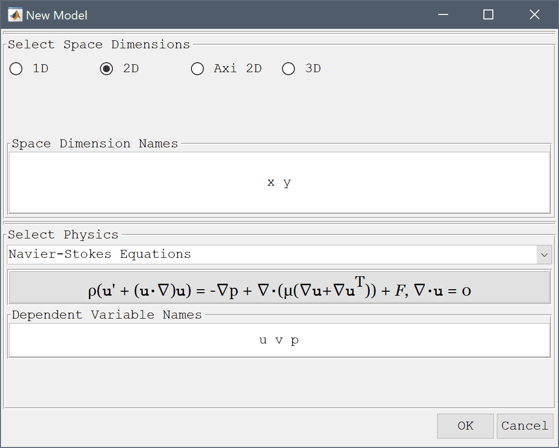
Select the Navier-Stokes Equations physics mode from the Select Physics drop-down menu.
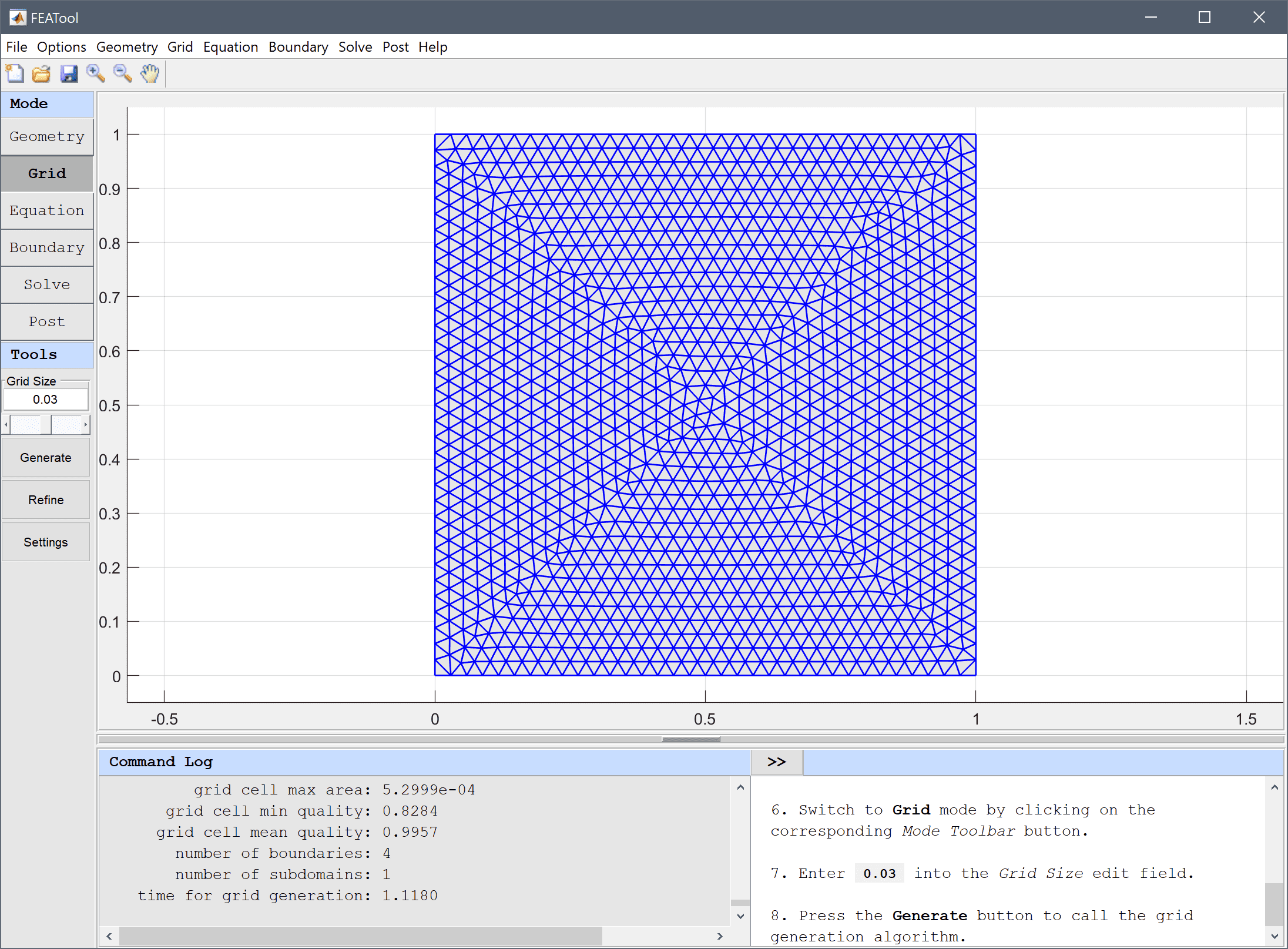
Enter 0.03 into the Grid Size edit field, and press the Generate button to call the grid generation algorithm.
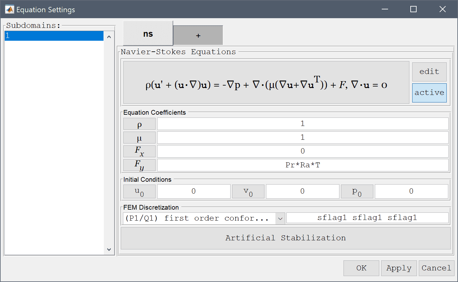
The non-dimensionalized form of the Boussinesq source term Pr·Ra·T couples the temperature to the y-direction source term of the Navier-Stokes equations.
Enter Pr*Ra*T into the Volume force in y-direction edit field.
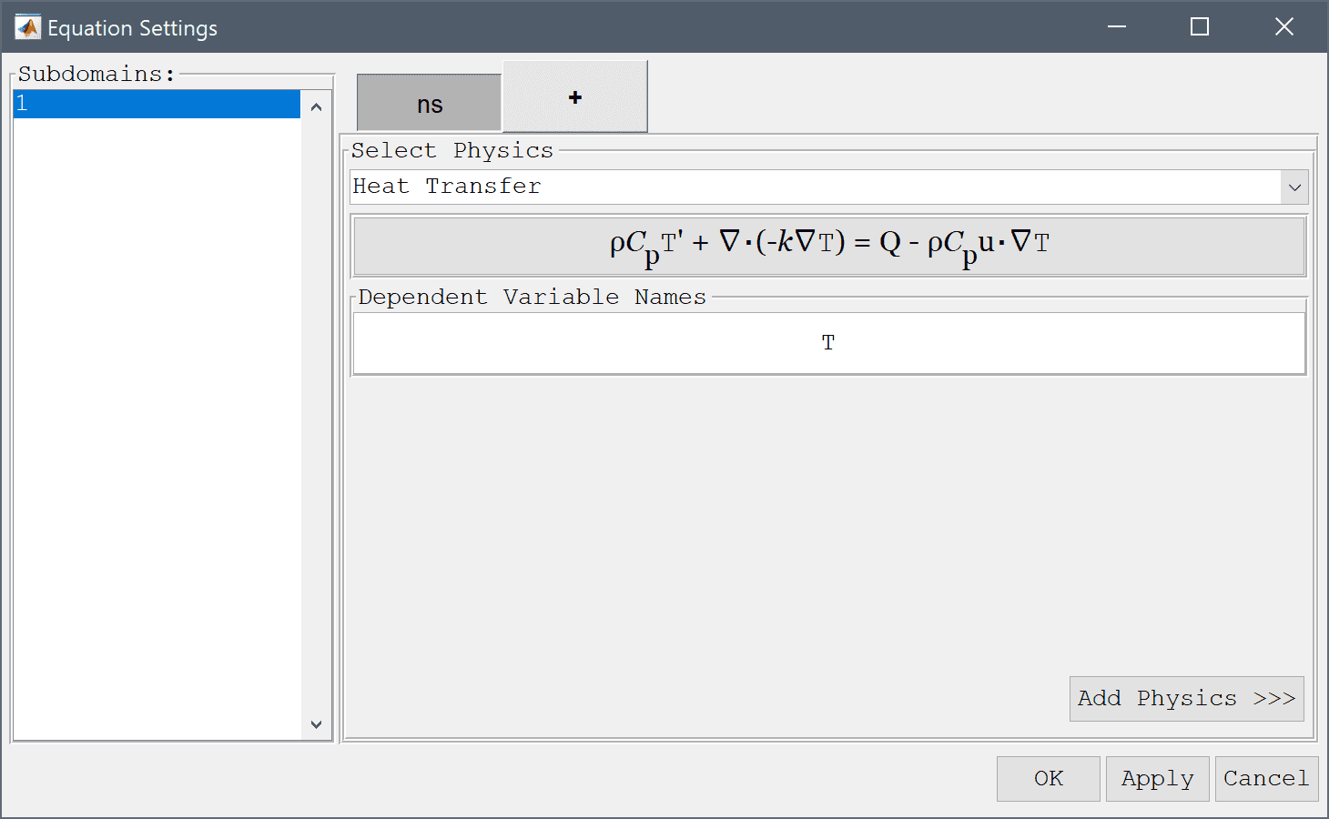
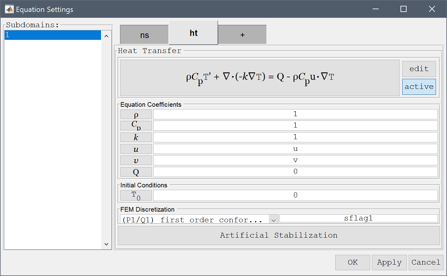
Add the heat transfer physics mode and coupled the velocities u and v to the convective transport terms.
Select the Heat Transfer physics mode from the Select Physics drop-down menu.
u into the Convection velocity in x-direction edit field.Enter v into the Convection velocity in y-direction edit field.
| Name | Expression |
|---|---|
| Pr | 0.71 |
| Ra | 1e3 |
Switch to the ns tab, which corresponds to the boundary conditions for the Navier-Stokes equations physics mode. Then select the Wall/no-slip for all four boundaries.
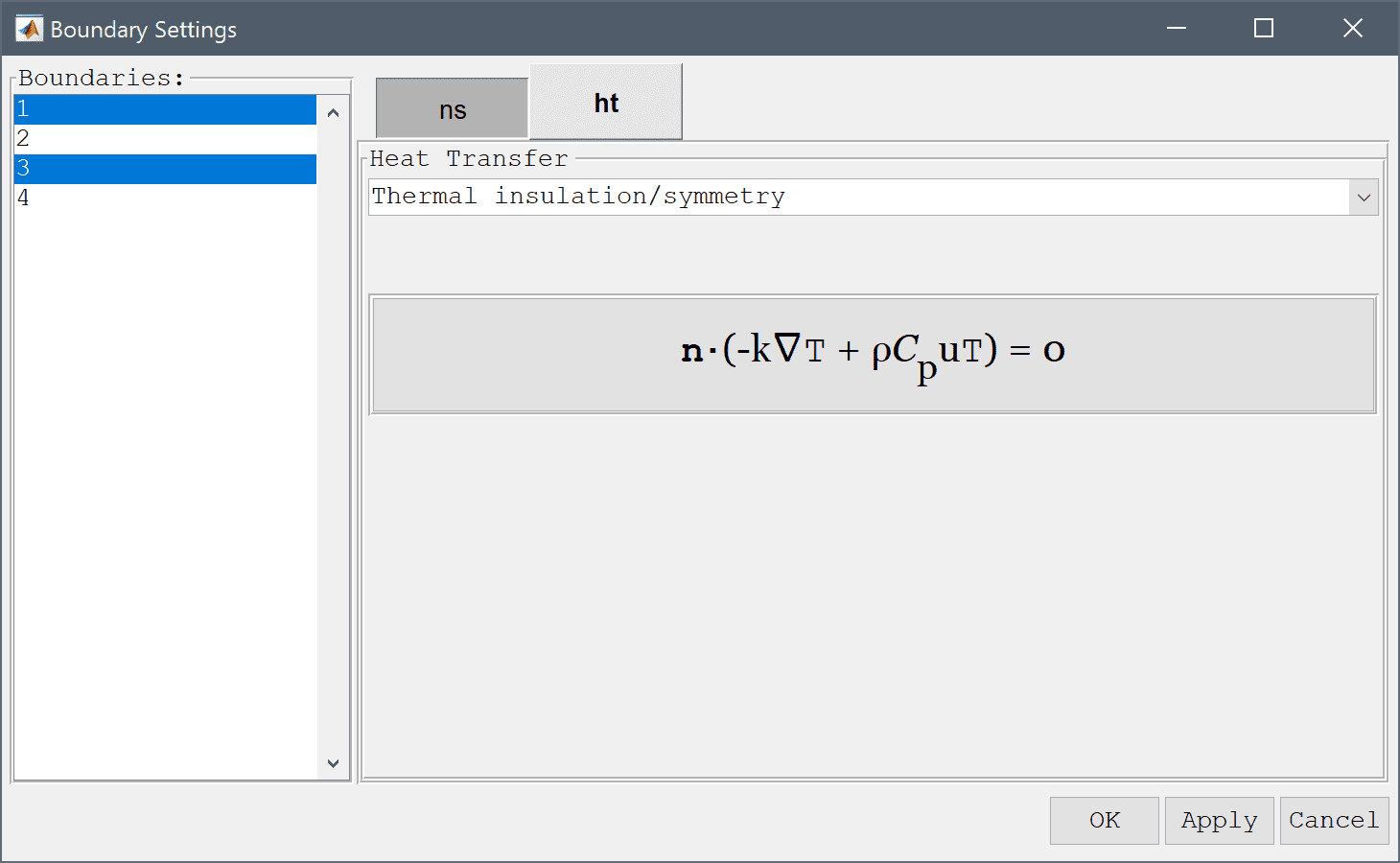
Click on the ht tab to change to specifying boundary conditions for the heat transfer physics mode. Select Thermal insulation/symmetry conditions for the top and bottom boundaries.
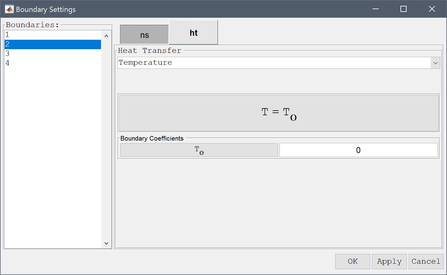
Select a Temperature boundary conditions for the left and right boundaries, and set a fixed temperature equal to 1 at the left side.
Enter 1 into the Temperature edit field.
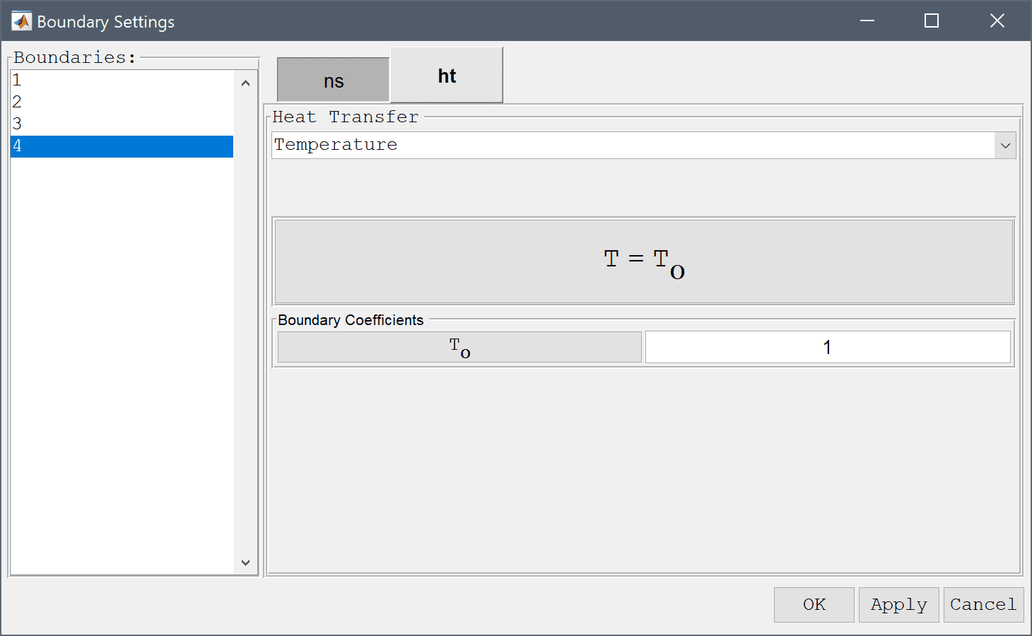
Select Temperature from the Heat Transfer drop-down menu.
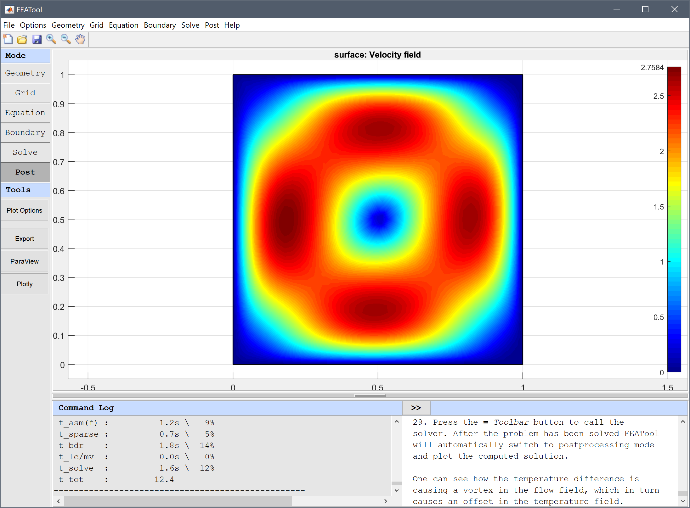
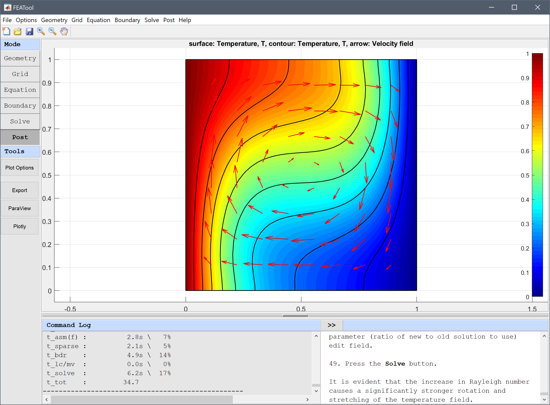
The solution shows how the temperature difference is causing a vortex in the flow field, which in turn causes an offset in the temperature field.
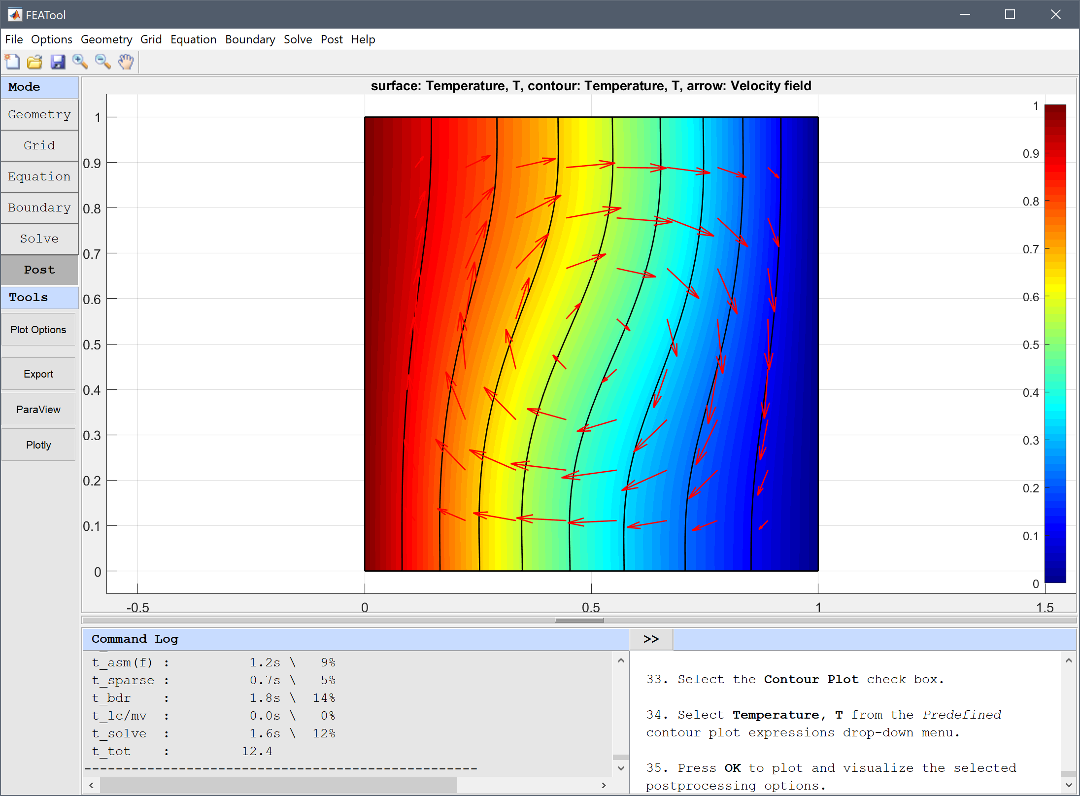
Change the plot to visualize the temperature field as surface and contour plots, and the velocity field as an arrow plot.
Select Temperature, T from the Predefined contour plot expressions drop-down menu.
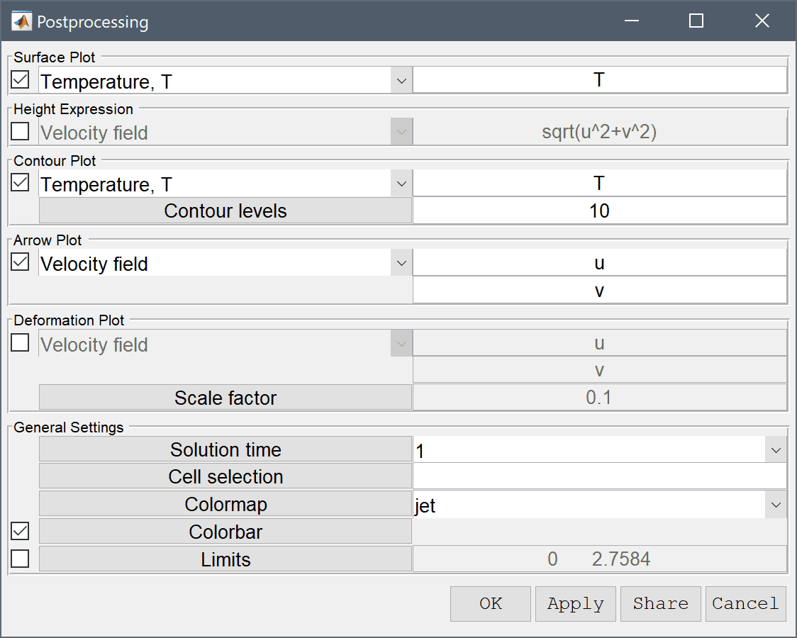
Press OK to plot and visualize the selected postprocessing options.
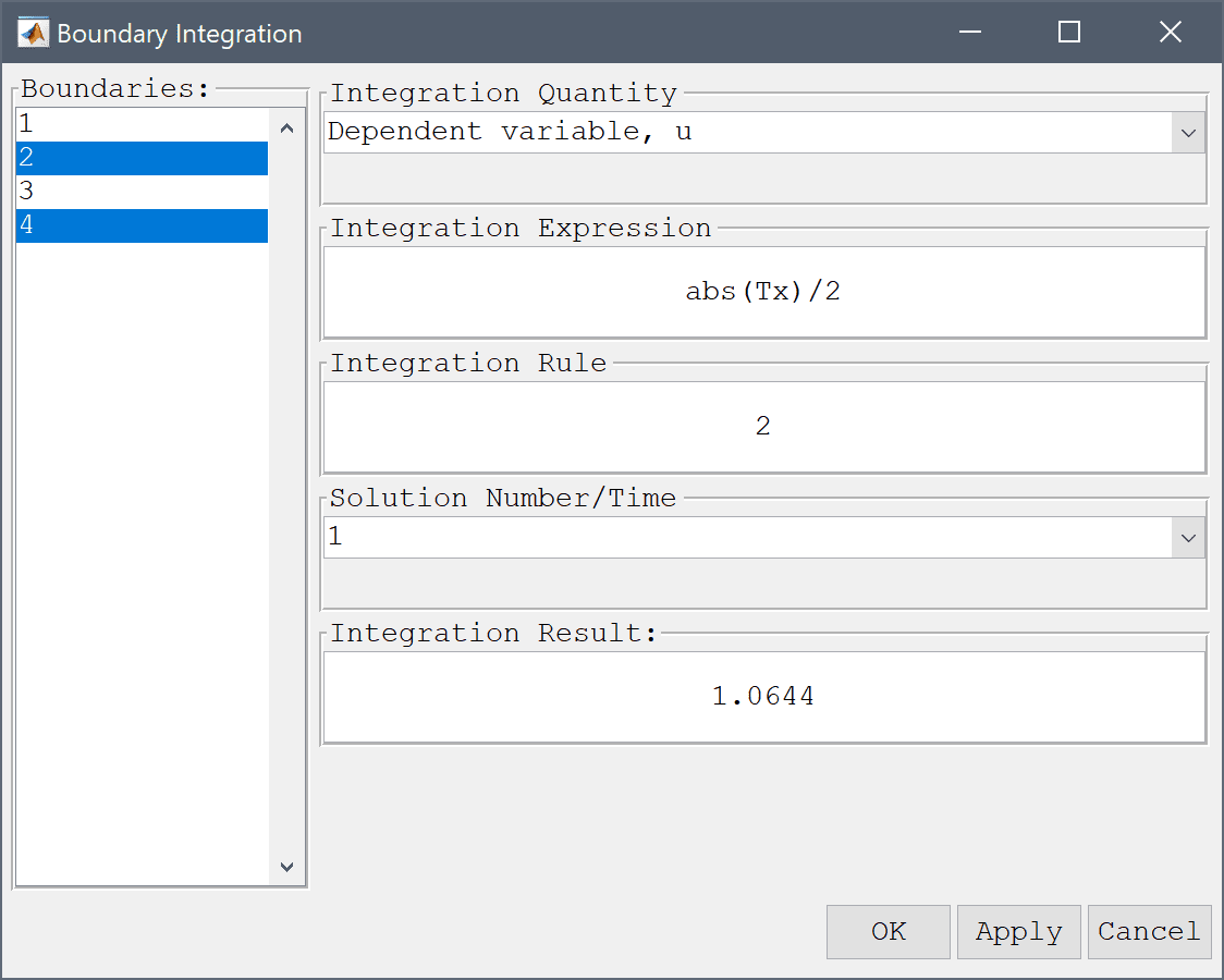
Use the boundary integration postprocessing tool to calculate the average Nusselt number for the vertical boundaries, and compare it to the reference value of 1.118.
abs(Tx)/2 into the Integration Expression edit field.Press OK to finish and close the dialog box.
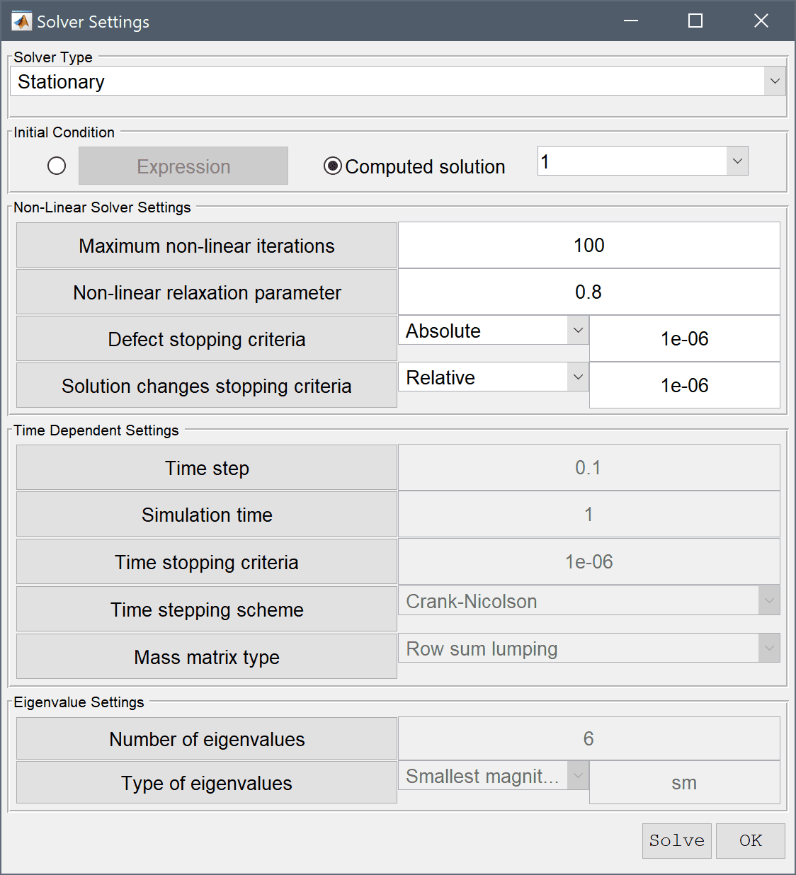
The simulation will now be repeated but with an increased Rayleigh number Ra = 104. Instead of starting over from the beginning the existing solution will be used as a starting guess which helps with non-linear convergence.
Enter 1e4 into the value field for Ra.
To assist with convergence, as well as selecting the old solution as initial value, also increase the non-linear relaxation and the maximum number of non-linear iterations.
100 into the Maximum number of non-linear iterations edit field.Enter 0.8 into the Non-linear relaxation parameter (ratio of new to old solution to use) edit field.
It is evident that the increase in Rayleigh number causes a significantly stronger rotation and stretching of the temperature field.
Use boundary integration tool again to calculate the mean Nusselt number for the vertical boundaries, and compare it to the corresponding reference value of 2.243 for Ra = 104.
Enter abs(Tx)/2 into the Integration Expression edit field.

The natural convection in a square cavity multiphysics model has now been completed and can be saved as a binary (.fea) model file, or exported as a programmable MATLAB m-script text file (available as the example ex_natural_convection script file), or GUI script (.fes) file.
[1] de Vahl D. Natural Convection of Air in a Square Cavity: A Benchmark Solution. Int. J. Numer. Meth. Fluids, vol. 3, pp. 249-264, 1983.
[2] de Vahl D, Jones IP. Natural Convection of Air in a Square Cavity: A Comparison Exercise. Int. J. Numer. Meth. Fluids, vol. 3, pp. 227-248, 1983.