This example describes how to model piezoelectric bending of a beam on the command line as an m-script model in FEATool. The test case comes from a research paper by Hwang and Park [3]. For this problem, the following coupled system of equations should be solved

\[ -\nabla\cdot \left[\begin{array}{c} \sigma \\ D \end{array}\right] = \left[\begin{array}{c} f \\ -\rho \end{array}\right] \]

where \(\sigma\) is a stress tensor, \(f\) represents body forces, \(D\) electric displacement, and \(\rho\) distributed charges.

By using the constitutive relations for a piezoelectric material [1], the stresses can in two dimensions be converted to the following form

\[ \nabla\cdot\left[ C \left[\begin{array}{c} \nabla u \\ \nabla v\ \\ \nabla V \end{array}\right]\right] = \left[\begin{array}{c} 0 \\ 0 \\ -\rho \end{array}\right] \]

where \(C\) is an array of constitutive relations and material parameters. This leads to a system of three equations for the unknown displacements \(u\) and \(v\), and the potential \(V\).

Tutorial

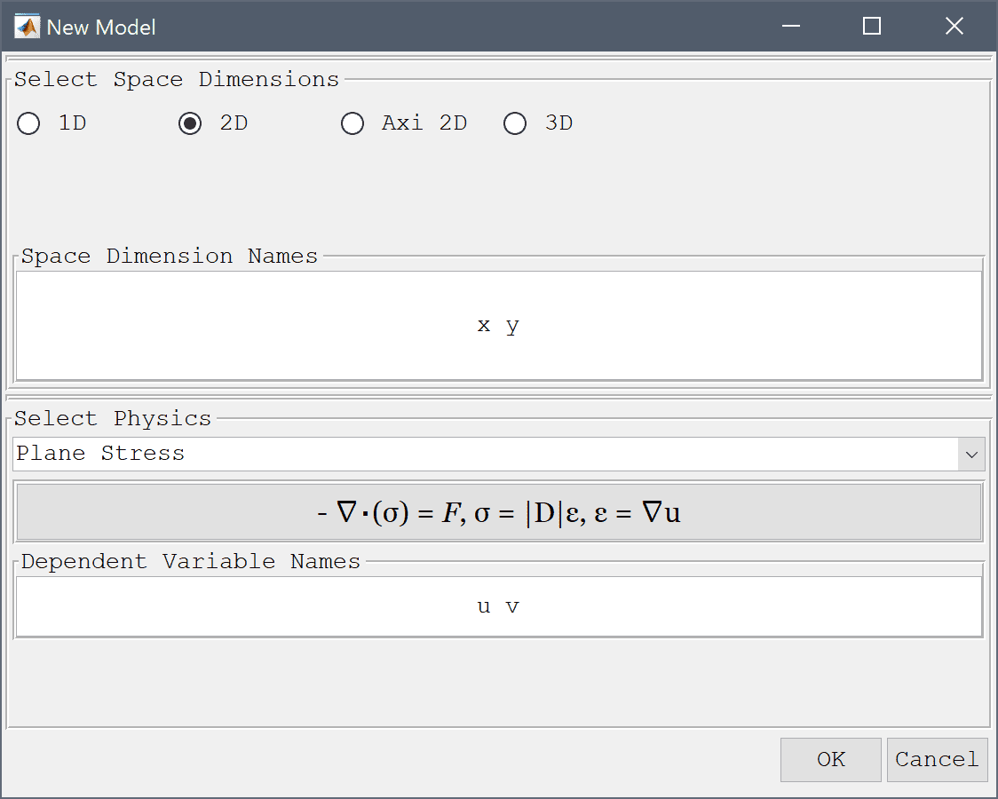
This model is available as an automated tutorial by selecting Model Examples and Tutorials... > Multiphysics > Piezo Electric Bending of a Beam from the File menu. Or alternatively, follow the step-by-step instructions below.

To start a new model click the New Model toolbar button, or select New Model... from the File menu.
Select the 2D radio button.
Select the Plane Stress physics mode from the Select Physics drop-down menu.
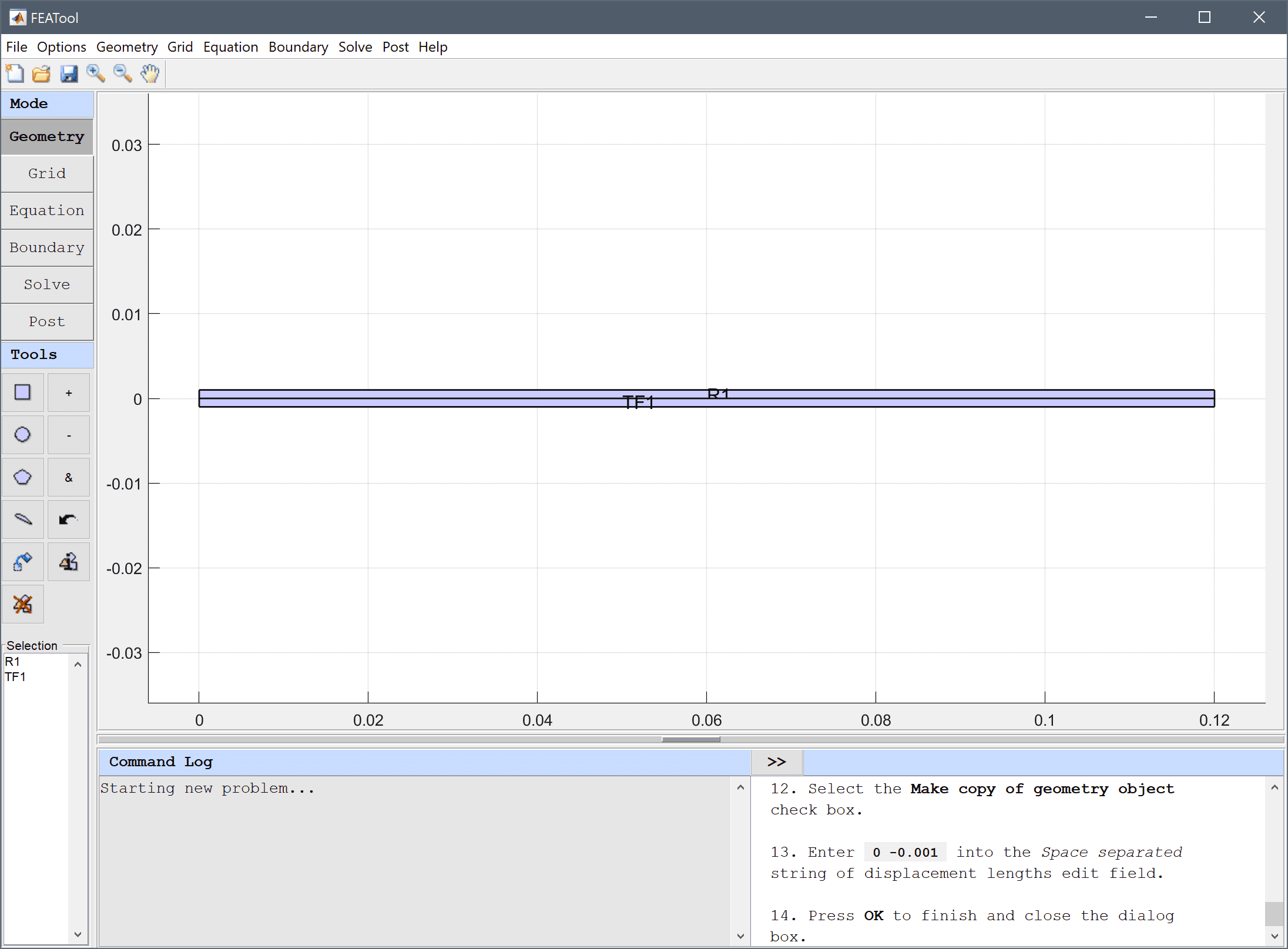
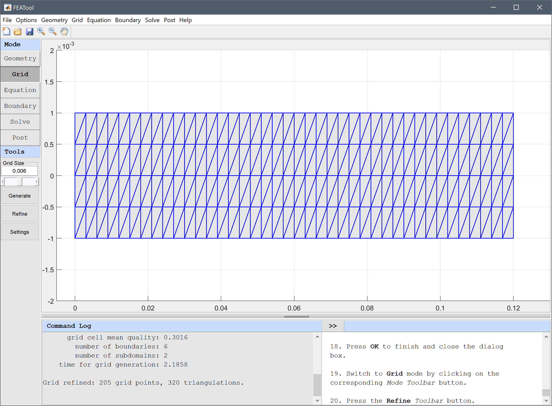
Press OK to finish the physics mode selection.

The beam consists of two 120 x 1 mm rectangular subdomains. First create the upper half and then copy it with a -1 mm offset.

Select Rectangle from the Geometry menu.
Enter 0.12 into the x_max edit field.
Enter 0 into the y_min edit field.
Enter 0.001 into the y_max edit field.
Press OK to finish and close the dialog box.
Select R1 in the geometry object Selection list box.
Press the Copy and/or transform selected geometry object Toolbar button.
Select the Make copy of geometry object check box.
Enter 0 -0.001 into the Space separated string of displacement lengths edit field.
Press OK to finish and close the dialog box.

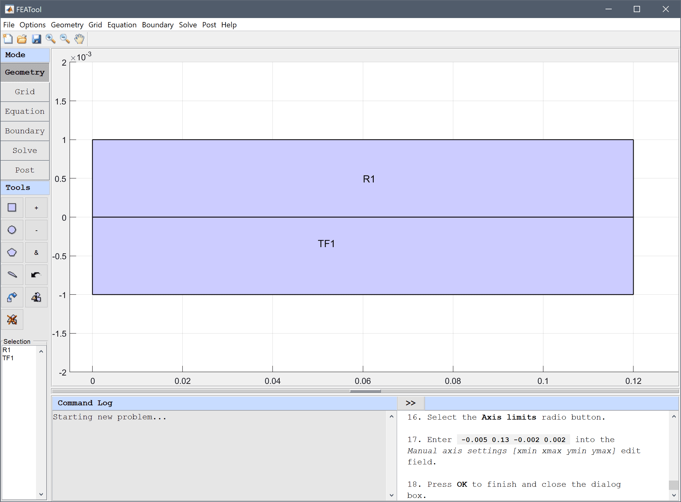
As the beam is very thin, manually change the axis ranges to see it better.

Select Axis/Grid Settings... from the Options menu.
Select the Axis limits radio button.
Enter -0.005 0.13 -0.002 0.002 into the Axis limits edit field.
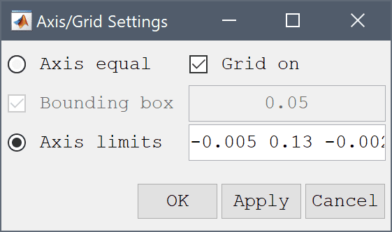
Press OK to finish and close the dialog box.
Switch to Grid mode by clicking on the corresponding Mode Toolbar button.
Press the Refine Toolbar button.
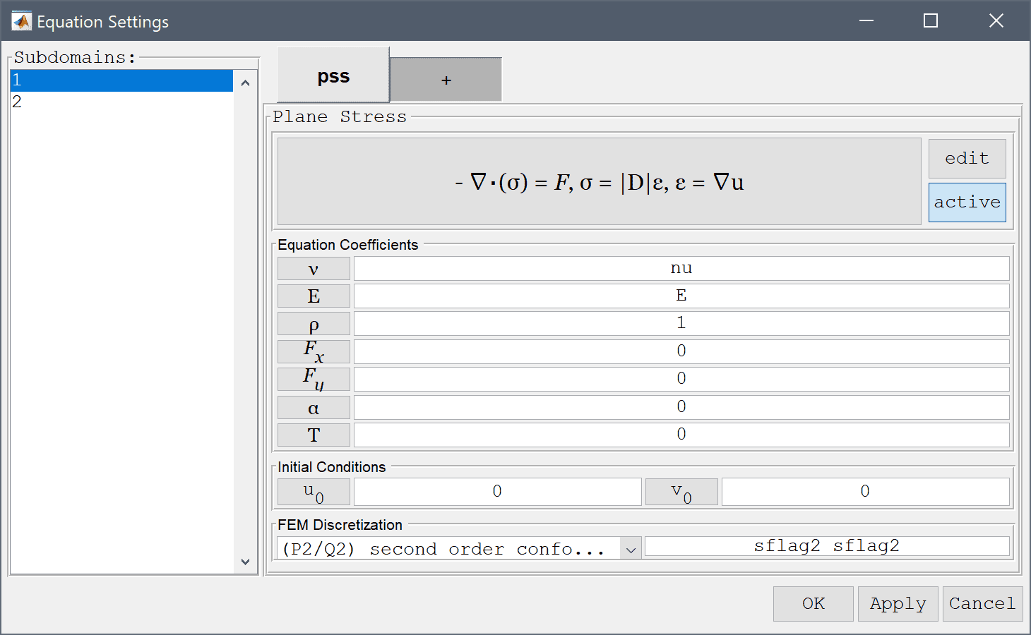
Switch to Equation mode by clicking on the corresponding Mode Toolbar button.
Enter nu into the Poisson's ratio edit field.
Enter E into the Modulus of elasticity edit field.

Second order accurate finite element shape functions are used for the displacement which are more accurate and allows for a coarser grid.

Select (P2/Q2) second order conforming from the FEM Discretization drop-down menu.
Press the edit button.

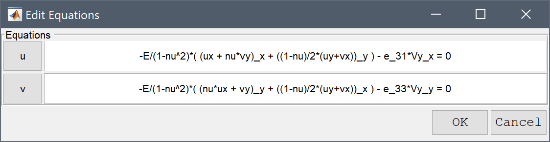
Open the edit equations dialog box and modify the plane-stress equations to include the coupling terms for the piezo-electric stress contributions, that is e31*Vyx and e31*Vyx.

Enter -E/(1-nu^2)*( (ux + nu*vy)_x + ((1-nu)/2*(uy+vx))_y ) - e_31*Vy_x = 0 into the Equation for u edit field.
Enter -E/(1-nu^2)*( (nu*ux + vy)_y + ((1-nu)/2*(uy+vx))_x ) - e_33*Vy_y = 0 into the Equation for v edit field.
Press OK to finish and close the dialog box.

Add the Conductive Media DC physics mode to account for the electrostatics effects.

Switch to the + tab.
Select the Conductive Media DC physics mode from the Select Physics drop-down menu.
Press the Add Physics >>> button.
Press the edit button.

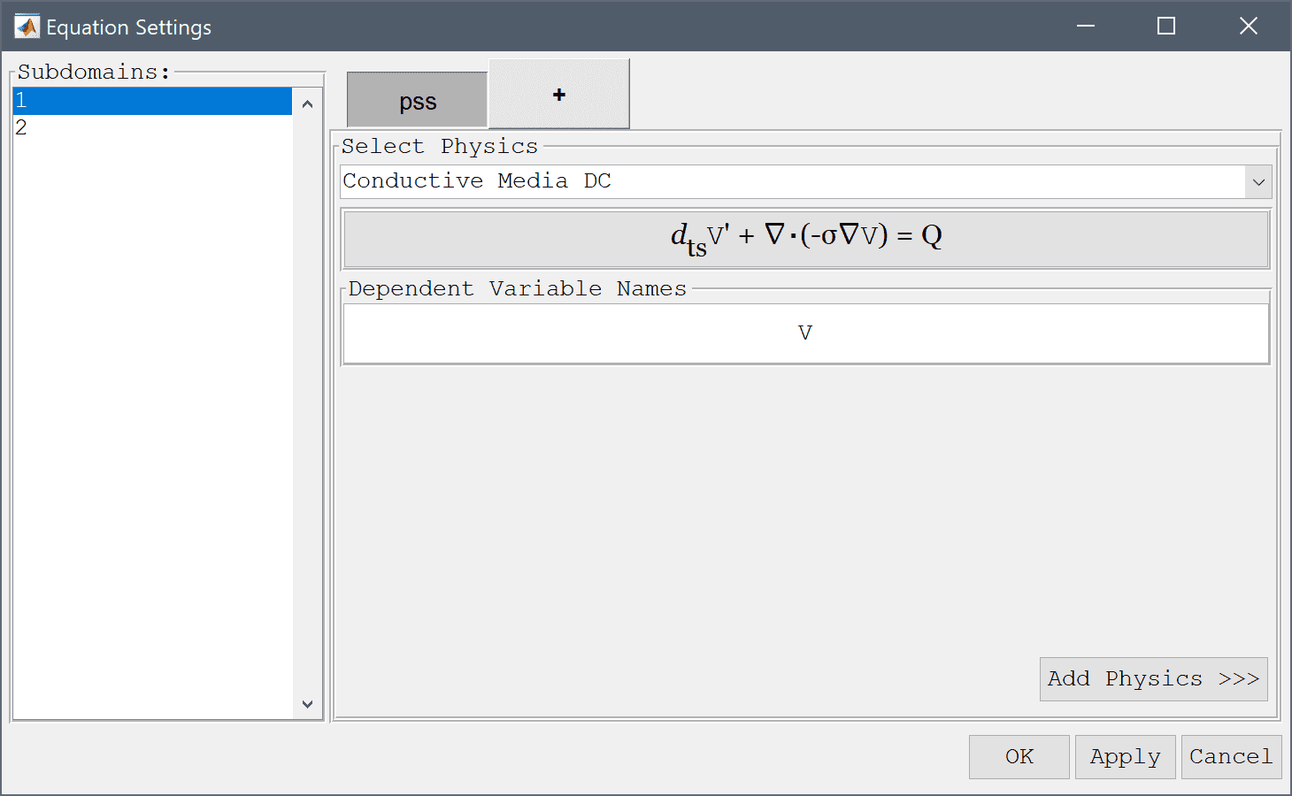
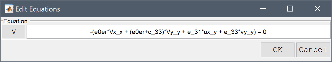
Again, change and modify the electrostatics equation to account for the piezo-electric effects.

Enter -(e0er*Vx_x + (e0er+c_33)*Vy_y + e_31*ux_y + e_33*vy_y) = 0 into the Equation for V edit field.
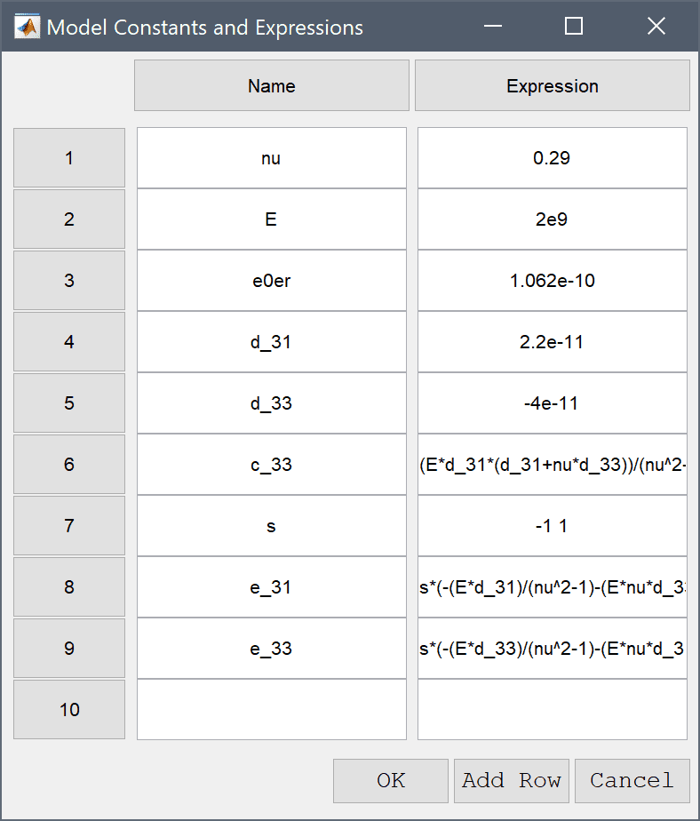
Press OK to finish equation editing and close the subdomain settings dialog box.
In order to define the piezo-electric modeling constants and expressions, press the Constants Toolbar button, or select the corresponding entry from the Equation menu, and enter the following variables in the Model Constants and Expressions dialog box. Note how the scaling factor s =-1 1 is used to invert the coefficients between the upper and lower halves. See the reference for more details.

Name	Expression
nu	0.29
E	2e9
e0er	1.062e-10
d_31	2.2e-11
d_33	-4e-11
c_33	(Ed_31(d_31+nud_33))/(nu^2-1)+(Ed_33(d_33+nud_31))/(nu^2-1)
s	-1 1
e_31	s(-(Ed_31)/(nu^2-1)-(Enud_33)/(nu^2-1))
e_33	s(-(Ed_33)/(nu^2-1)-(Enud_31)/(nu^2-1))

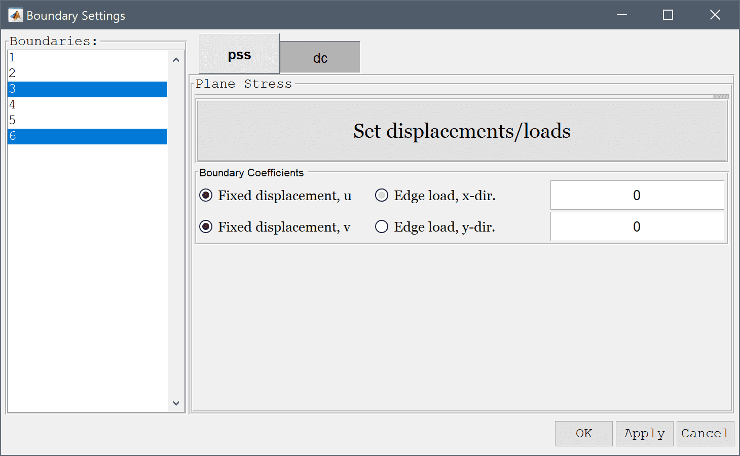
Switch to Boundary mode by clicking on the corresponding Mode Toolbar button.

The beam is considered fixed at the left end, which means constrained displacements in all directions.

Select 3 and 6 in the Boundaries list box.
Select the Fixed displacement, v radio button.
Select the Fixed displacement, u radio button.
Switch to the dc tab.
Select 2 in the Boundaries list box.

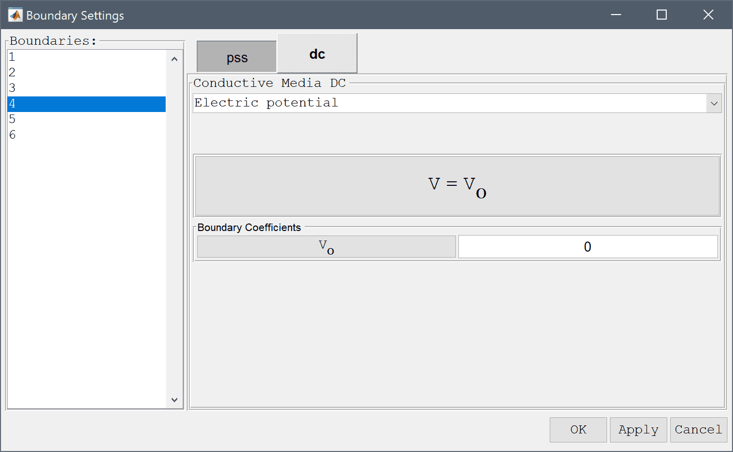
A voltage difference of 250 V is applied between the top and bottom boundaries.

Select Electric potential from the Conductive Media DC drop-down menu.
Enter 250 into the Electric potential edit field.
Select 4 in the Boundaries list box.
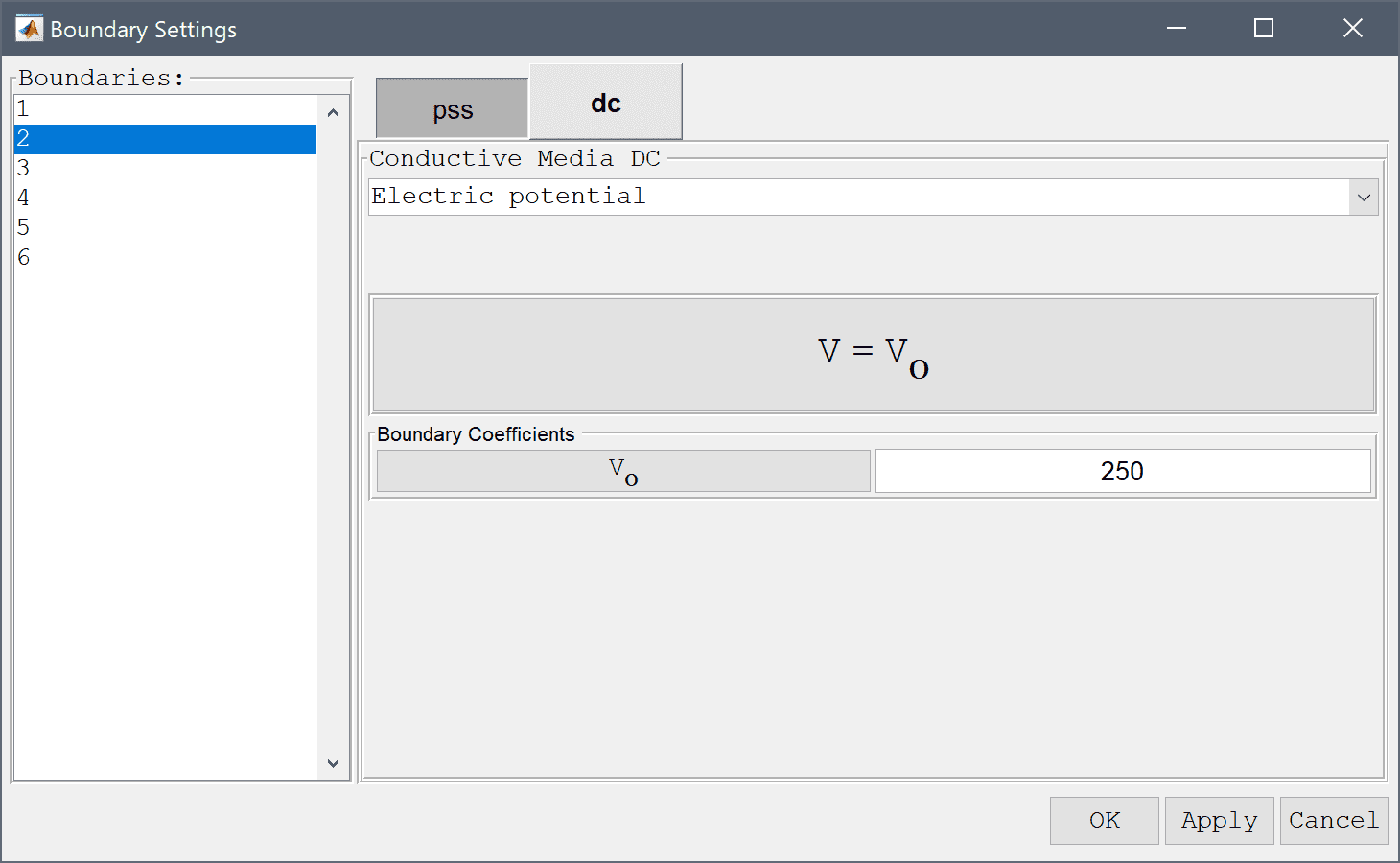
Select Electric potential from the Conductive Media DC drop-down menu.
Press OK to finish the boundary condition specification.
Switch to Solve mode by clicking on the corresponding Mode Toolbar button.
Press the = Toolbar button to call the solver. After the problem has been solved FEATool will automatically switch to postprocessing mode and plot the computed solution.

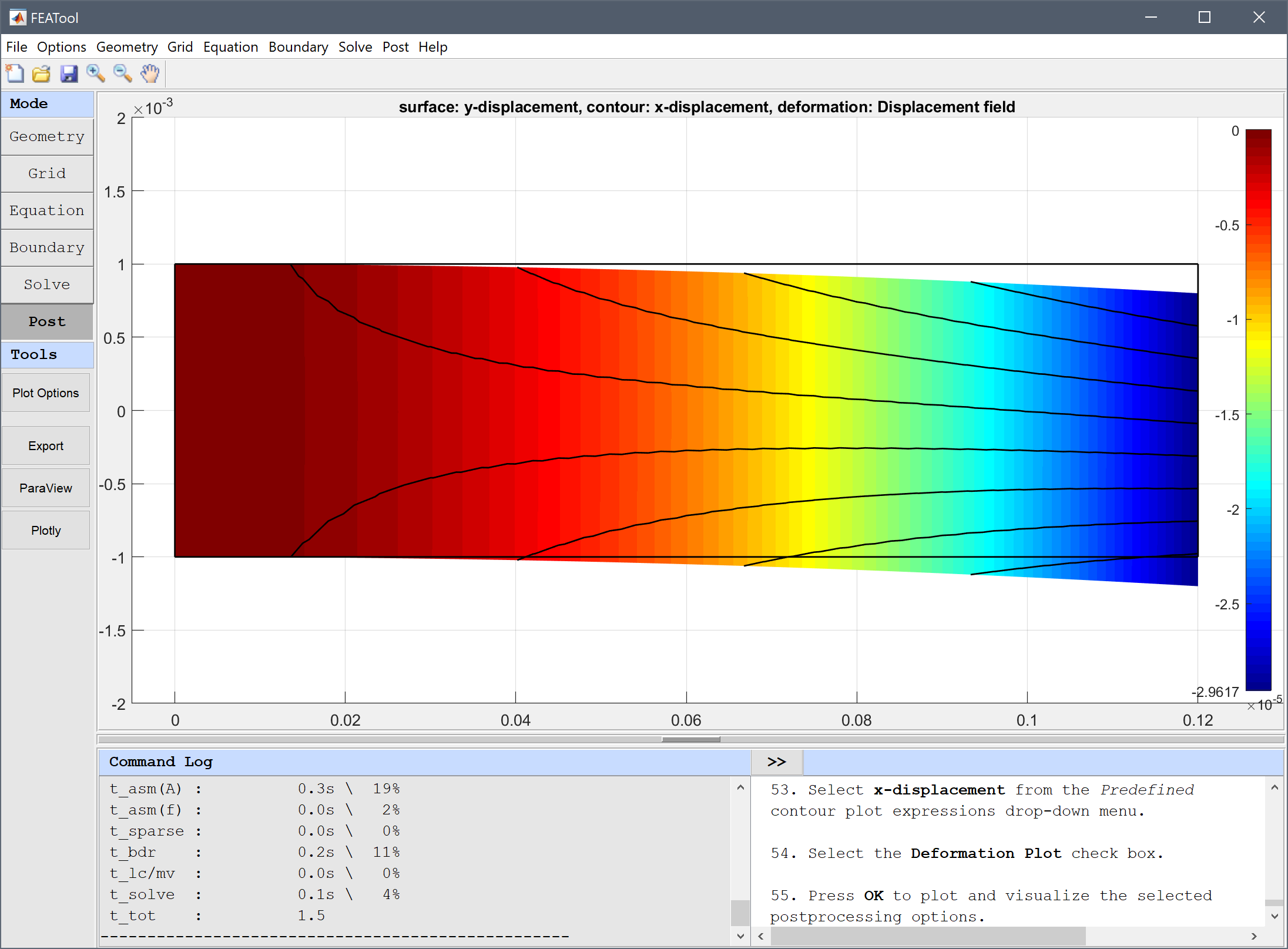
Plot and visualize the displacement in the y-direction. The maximum displacement it around 29.6 µm which agrees well with the theoretically expected solution.

Press the Plot Options Toolbar button.
Select y-displacement from the Predefined surface plot expressions drop-down menu.
Select the Contour Plot check box.
Select x-displacement from the Predefined contour plot expressions drop-down menu.
Select the Deformation Plot check box.
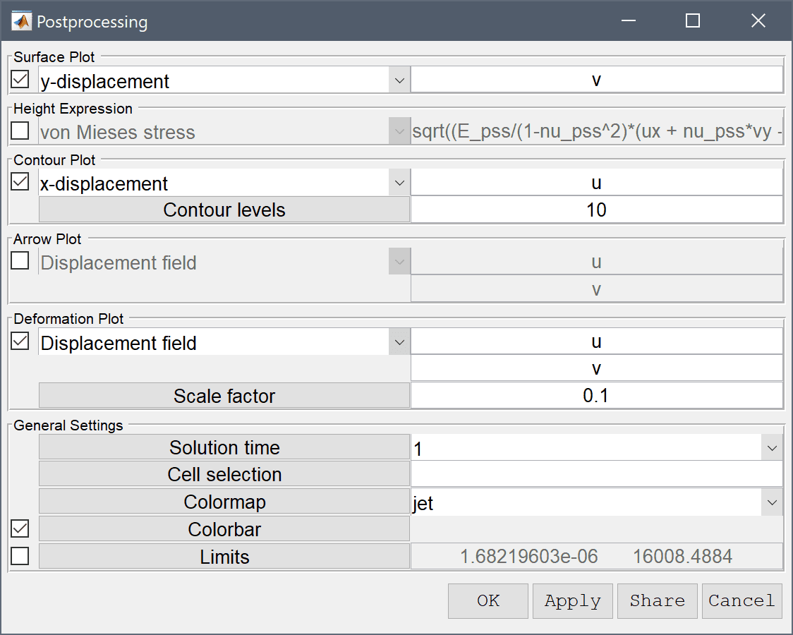
Press OK to plot and visualize the selected postprocessing options.

The piezo electric bending of a beam multiphysics model has now been completed and can be saved as a binary (.fea) model file, or exported as a programmable MATLAB m-script text file, or GUI script (.fes) file.

CLI Tutorial

In this section the model is defined and solved as a MATLAB m-script file. Here we will be looking at composition of two 1.2 cm long and 2 mm thick beams with opposite polarization.

First we assign names to the space coordinates (x and y), and create a grid. Note, that the shape is so simple here that we don't need to explicitly define a geometry, we can use the 'rectgrid' command directly

fea.sdim = { 'x' 'y' };
fea.grid = rectgrid( 20, 20, [ 0 12e-3; -1e-3 1e-3] );

Next is to define the equation coefficients and constitutive relations. See the attached file for their definitions, one thing to note that to define the polarization the coefficient is multiplied with a switch expression 2*(y<0)-1 which evaluates to 1 in the top half and -1 in the bottom (here we have also used the name y for the space coordinate in the 2nd direction as we defined earlier).

Now we define the dependent variables and assign 2nd order Lagrange finite element shape functions for them all

fea.dvar  = { 'u' 'v' 'V' };
fea.sfun  = { 'sflag2' 'sflag2' 'sflag2' };

The material parameters and constitutive relations are defined as

% Equation coefficients.
Emod =  2e9;       % Modulus of elasticity
nu   =  0.29;      % Poissons ratio
Gmod =  0.775e9;   % Shear modulus
d31  =  0.22e-10;  % Piezoelectric sn coefficient
d33  = -0.3e-10;   % Piezoelectric sn coefficient
prel = 12;         % Relative electrical permittivity
pvac = 0.885418781762-11; % Elec. perm. of vacuum

% Constitutive relations.
constrel   = [ Emod/(1-nu^2)    nu*Emod/(1-nu^2) 0    ;
               nu*Emod/(1-nu^2) Emod/(1-nu^2)    0    ;
               0                0                Gmod ];
piezoel_st = [ 0 d31 ;
               0 d33 ;
               0 0   ];
piezoel_sn = constrel*piezoel_st;
dielmat_st = [ prel 0    ;
               0    prel ]*pvac ;
dielmat_sn = [ dielmat_st - piezoel_st'*piezoel_sn ];

% Populate coefficient matrices (negative sign
% due to fem partial integration).
c{1,1} = { constrel(1,1)   constrel(1,3) ;
           constrel(1,3)   constrel(3,3) };
c{1,2} = { constrel(1,3)   constrel(1,2) ;
           constrel(3,3)   constrel(2,3) };
c{2,1} = c{1,2}';
c{2,2} = { constrel(3,3)   constrel(1,3) ;
           constrel(1,3)   constrel(2,2) };
c{1,3} = { piezoel_sn(1,1) piezoel_sn(1,2) ;
           piezoel_sn(3,1) piezoel_sn(3,2) };
for i=1:4
  c{1,3}{i} = [num2str(c{1,3}{i}),'*(2*(y<0)-1)'];
end
c{3,1} = c{1,3}';
c{2,3} = { piezoel_sn(3,1) piezoel_sn(3,2);
           piezoel_sn(2,1) piezoel_sn(2,2) };
for i=1:4
  c{2,3}{i} = [num2str(c{2,3}{i}),'*(2*(y<0)-1)'];
end
c{3,2} = c{2,3}';
c{3,3} = { dielmat_sn(1,1) dielmat_sn(2,1) ;
           dielmat_sn(2,1) dielmat_sn(2,2) };

To define the finite element bilinear forms we use the following code

bilinear_form = [ 2 2 3 3 ;
                  2 3 2 3 ];
for i=1:length(fea.dvar)
  for j=1:length(fea.dvar)
    fea.eqn.a.form{i,j} = bilinear_form;
    fea.eqn.a.coef{i,j} = c{i,j}(:)';
   end
end

where each bilinear form has four terms, the top line in the definition defines the finite element shape for the dependent variable, and second line for the test function space (a 2 indicates x-derivative, and 3 y-derivative).

In this case all three source terms are zero, thus

fea.eqn.f.form = { 1 1 1 };
fea.eqn.f.coef = { 0 0 0 };

The boundary conditions are defined as follows

n_bdr                   = max(fea.grid.b(3,:));
fea.bdr.d               = cell(3,n_bdr);
fea.bdr.n               = cell(3,n_bdr);
i_top                   = 3;
i_bottom                = 1;
i_left                  = 4;
[fea.bdr.d{3,i_top}]    = deal( 200 );
[fea.bdr.d{3,i_bottom}] = deal( 0 );
[fea.bdr.d{1:2,i_left}] = deal( 0 );

In this way we have set a potential difference of 200, and fixed the left hand side boundary. Now we parse the problem struct and solve the system with

fea       = parseprob( fea );
fea.sol.u = solvestat( fea );

After the problem has been solved we can for example visualize the displacement in the y-direction with the following command

postplot( fea, 'surfexpr', 'v', ...
               'isoexpr',  'u', ...
               'deformexpr', { 'u', 'v' } )

An example m-script file for this model can be found in the ex_piezoelectric1 m-script file.

CLI Postprocessing

To visualize the full 3D solution from the planar model, the data can be exported and processed on the MATLAB command line interface (CLI) console with the Export Model Data Struct to MATLAB option from the File menu. The postextrude and postplot functions can then be applied to extrude and visualize the data, for example

fea_extruded = postextrude( fea, 5, 6e-3 );

postplot( fea_extruded, 'surfexpr', 'u', 'deformexpr', {'u', 0, 'v'}, ...
          'parent', figure )

colorbar off
axis off
axis normal
axis( [ 0, 0.121, -20e-3, 20e-3, -20e-3, 20e-3 ] )
view( 33, 24 )

References

[1] Tseng CI. Electromechanical Dynamics of a Coupled Piezo-electric/Mechanical System Applied to Vibration Control and Distributed Sensing. Univ. of Kentucky, Lexington, 1989.

[2] Pierfort V. Finite Element Modeling of Piezoelectric Active Structures. ULB, Faculty of Applied Sciences, 2000.

[3] Hwang WS, Park HC. Finite Element Modeling of Piezoelectric Sensors and Actuators. AIAA Journal, Vol. 31, No. 5, 1993.