Thermo-Mechanical Bending of a Beam

Coupled thermo-mechanical multiphysics simulation of bending of a cantilever beam. The left side of the beam is fixed to a solid wall while the top side is subjected to an elevated external temperature through natural convection. The lower and left side are continuously held at the initial zero temperature. A two-dimensional plane stress approximation is also used, where the material is assumed to have a Poisson ratio of 0.25, modulus of elasticity 30 GPa, and convective heat transfer coefficient 10 W/m/K. All other coefficients are assumed to be equal to one. The temperature influx from the top boundary causes an increased internal temperature and also results in a downward deflection of the beam. After 10 seconds the top surface temperature has risen to 5 degrees and the beam has bent around 0.5-0.6 mm downwards.

Tutorial

This model is available as an automated tutorial by selecting Model Examples and Tutorials... > Multiphysics > Thermo-Mechanical Bending of a Beam from the File menu. Or alternatively, follow the step-by-step instructions below.

1. To start a new model click the New Model toolbar button, or select New Model... from the File menu.
2. Select the Plane Stress physics mode from the Select Physics drop-down menu.
3. Press OK to finish the physics mode selection.

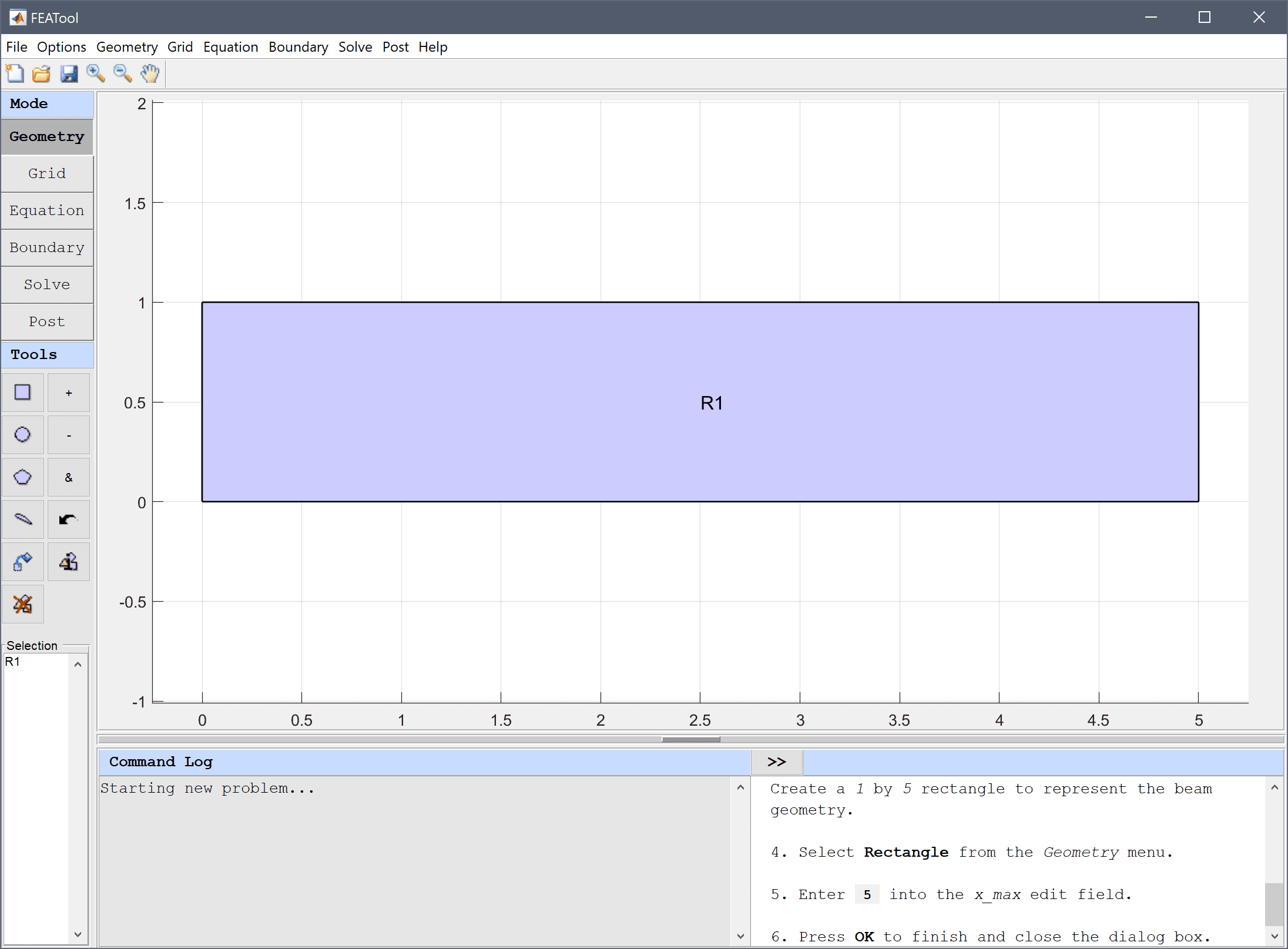
Create a 1 by 5 rectangle to represent the beam geometry.

1. Select Rectangle from the Geometry menu.
2. Enter 5 into the x_max edit field.

3. Press OK to finish and close the dialog box.

   
4. Switch to Grid mode by clicking on the corresponding Mode Toolbar button.
5. Switch to Equation mode by clicking on the corresponding Mode Toolbar button.

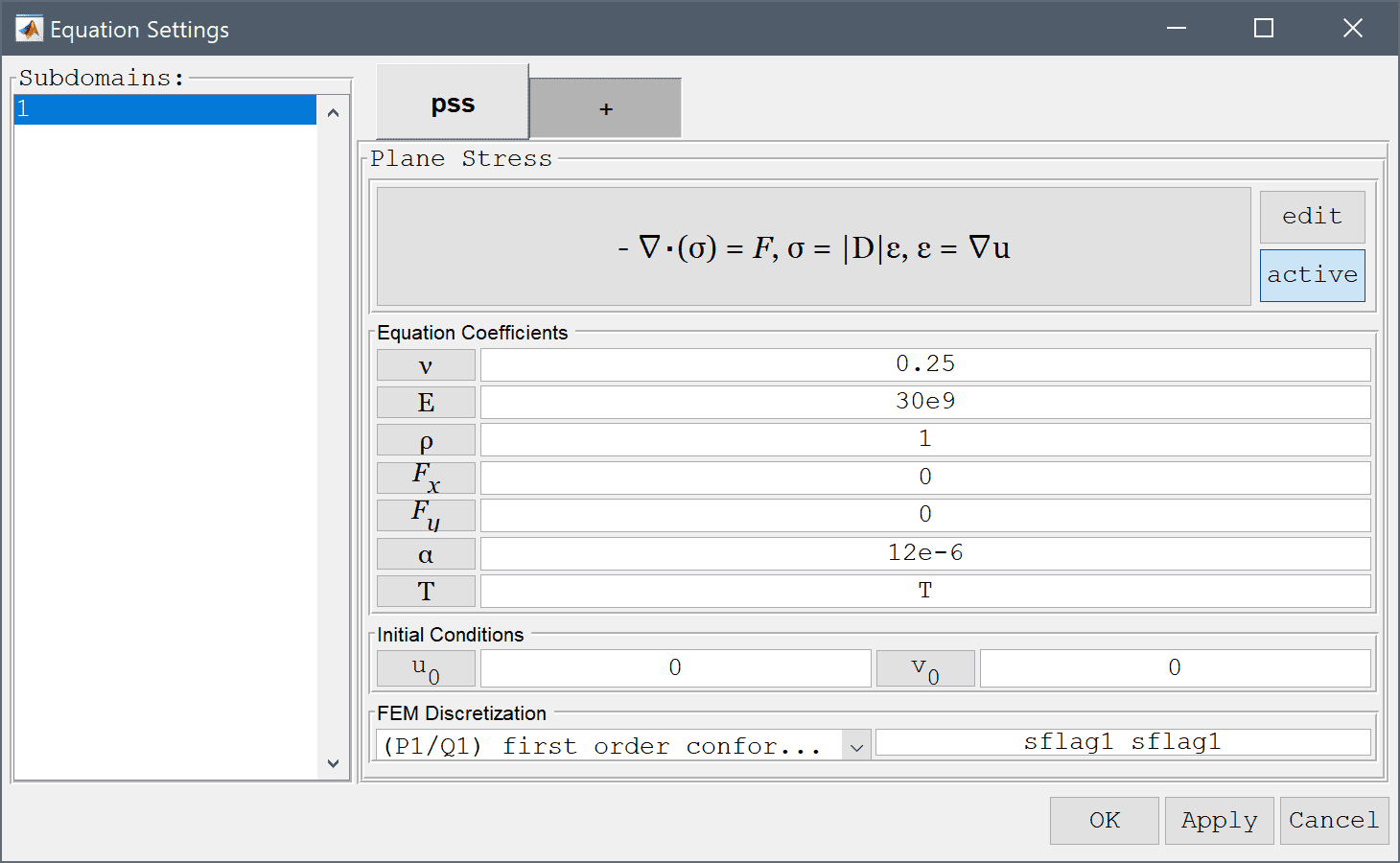
The material is assumed to have a Poisson ratio of 0.25, modulus of elasticity 30 GPa, and zero initial temperature. All other coefficients are assumed to be equal to one.

1. Enter 0.25 into the Poisson's ratio edit field.
2. Enter 30e9 into the Modulus of elasticity edit field.
3. Enter 12e-6 into the Thermal expansion coefficient edit field.

4. Enter T into the Temperature edit field.

   
5. Switch to the + tab.
6. Select the Heat Transfer physics mode from the Select Physics drop-down menu.
7. Press the Add Physics >>> button.
8. Press OK to finish the equation and subdomain settings specification.
9. Switch to Boundary mode by clicking on the corresponding Mode Toolbar button.

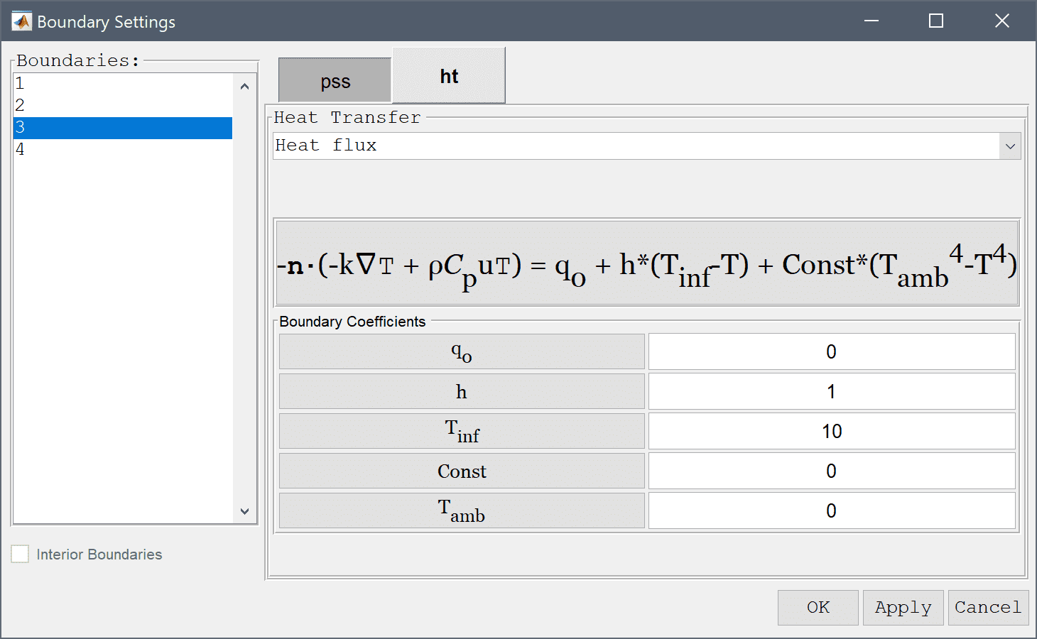
The left side of the beam is fixed to a solid wall while the top side is subjected to an elevated external temperature through natural convection with a heat transfer coefficient 10 W/m/K.

1. Select 4 in the Boundaries list box.
2. Select the Fixed displacement, u radio button.
3. Select the Fixed displacement, v radio button.
4. Switch to the ht tab.
5. Select 1 and 4 in the Boundaries list box.
6. Select Temperature from the Heat Transfer drop-down menu.
7. Select 3 in the Boundaries list box.
8. Select Heat flux from the Heat Transfer drop-down menu.
9. Enter 10 into the Bulk temperature edit field.

10. Enter 1 into the Heat transfer coefficient edit field.

    
11. Press OK to finish the boundary condition specification.
12. Switch to Solve mode by clicking on the corresponding Mode Toolbar button.

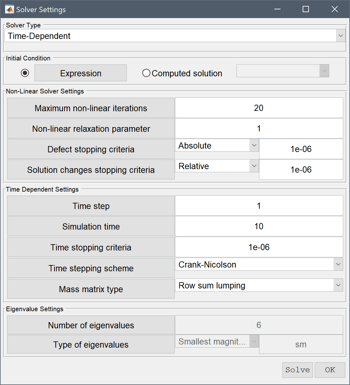
Open the Solver Settings dialog box, set the Time Step to 1, and Simulation Time to 10.

1. Press the Settings Toolbar button.
2. Select Time-Dependent from the Solution and solver type drop-down menu.
3. Enter 1 into the Time step size edit field.

4. Enter 10 into the Duration of time-dependent simulation (maximum time) edit field.

   
5. Press the Solve button.

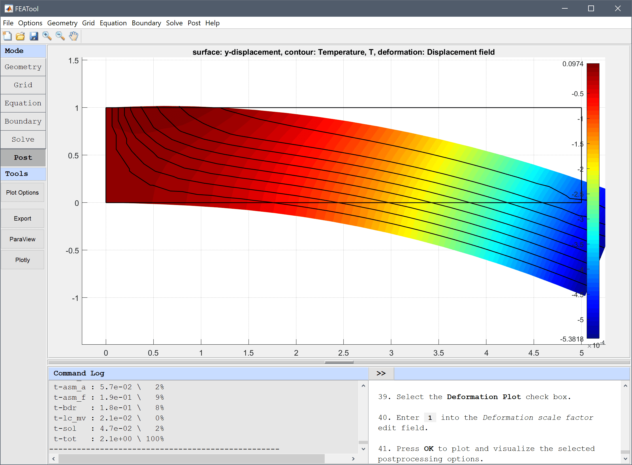
Plot and visualize the displacement in the y-direction and temperature.

After 10 seconds the top surface temperature has risen by 5 degrees and the beam has bent around 0.5-0.6 mm downwards.

1. Press the Plot Options Toolbar button.
2. Select y-displacement from the Predefined surface plot expressions drop-down menu.
3. Select the Contour Plot check box.
4. Select Temperature, T from the Predefined contour plot expressions drop-down menu.

5. Select the Deformation Plot check box.

   

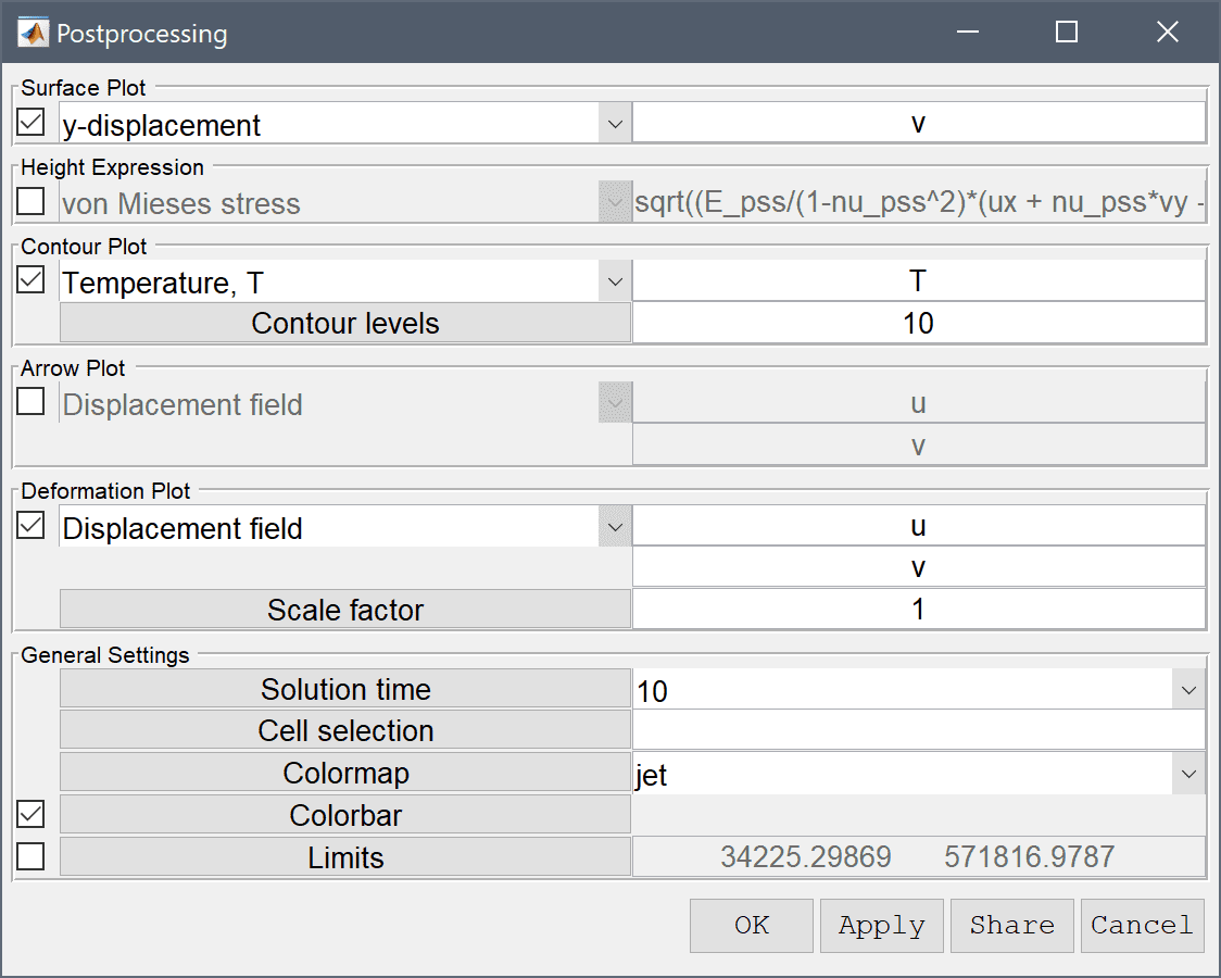
6. Press OK to plot and visualize the selected postprocessing options.

   

The thermo-mechanical bending of a beam multiphysics model has now been completed and can be saved as a binary (.fea) model file, or exported as a programmable MATLAB m-script text file, or GUI script (.fes) file.