|
|
FEATool Multiphysics
v1.18.0
Finite Element Analysis Toolbox
|
|
|
FEATool Multiphysics
v1.18.0
Finite Element Analysis Toolbox
|
Fluid-structure interaction benchmark problem for stationary, laminar, and incompressible flow around a cylinder with an attached elastic beam. Although it is not possible to derive an analytical solution to these test cases, numerical solutions to benchmark reference quantities have been established for the beam deformation, drag, and lift forces [1].
The test configurations consider a solid cylinder centered at (0.2, 0.2) with diameter d = 0.1 in a l = 2.2 by h = 0.41 rectangular channel. The fluid is assumed to have a constant density and viscosity, and a fully developed parabolic velocity profile is prescribed at the inlet. A beam of length 0.4 and width 0.02 is fixed to the end of the cylinder. First a static solution with a Reynolds number Re = 20 is considered, and then an instationary solution with Re = 100.
This model is available as an automated tutorial by selecting Model Examples and Tutorials... > Multiphysics > Fluid-Structure Interaction - Elastic Beam from the File menu. Or alternatively, follow the step-by-step instructions below.
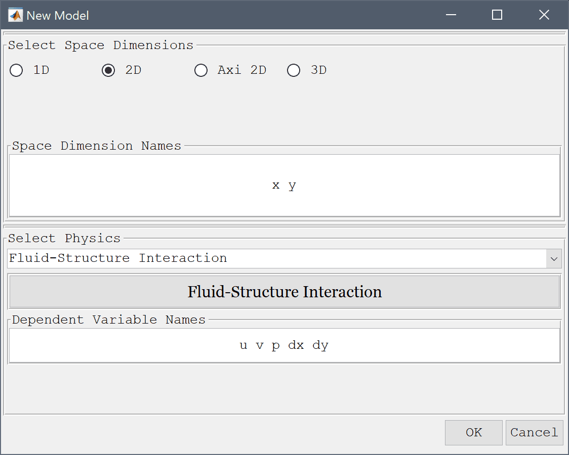
In the New Model dialog box, select 2D for the Space Dimensions, and select Fluid-Structure Interaction from the Select Physics drop-down menu. Leave the space dimension and dependent variable names to their defaults and press OK to finish the physics mode selection.
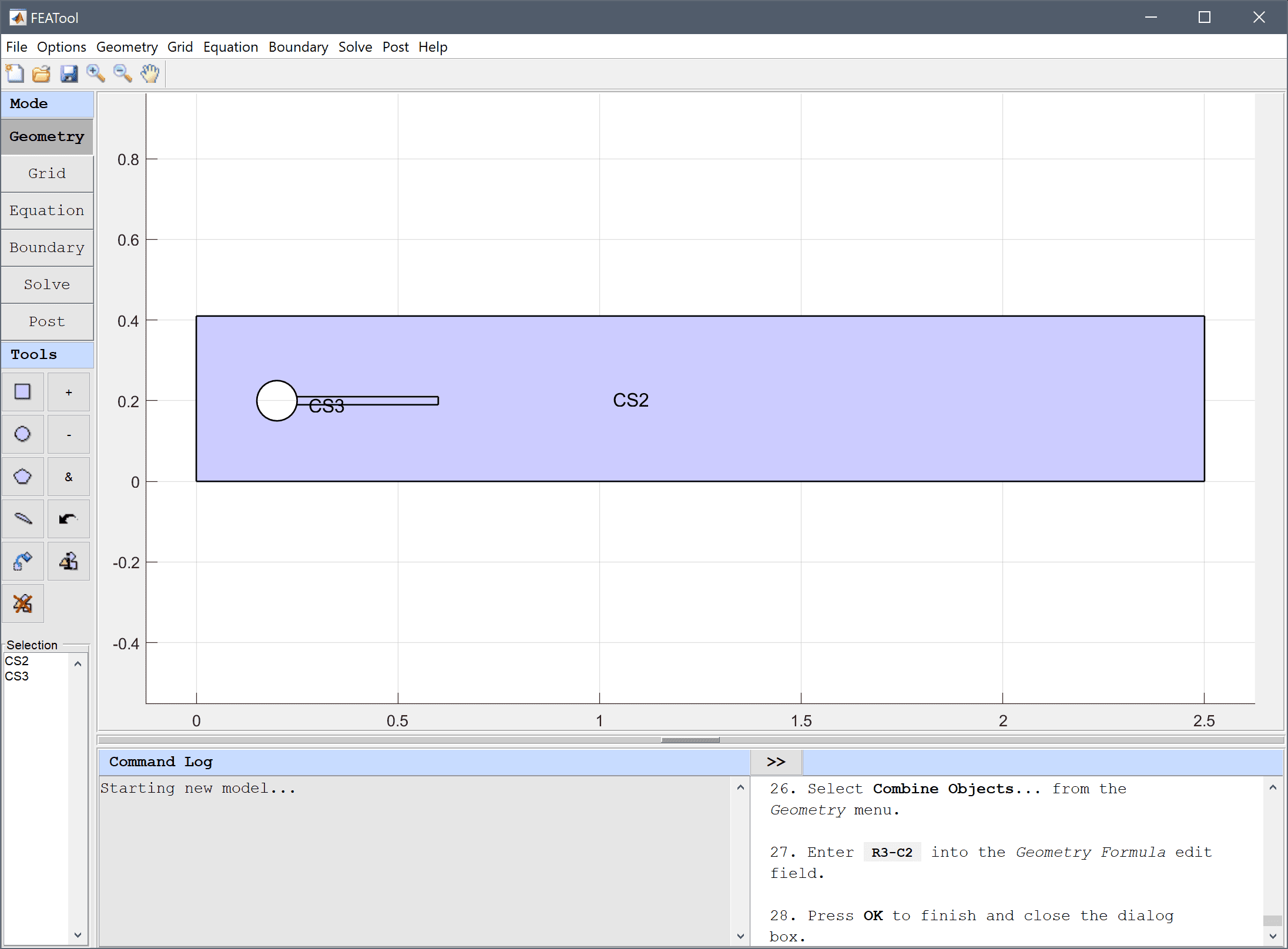
The geometry consists of two subdomains, an outer 0.41 by 2.5 rectangle with a circular hole centered at (0.2, 0.2), and a 0.4 by 0.02 thin rectangular beam.
Start with selecting Rectangle from the Geometry menu.
2.5 into the xmax edit field.0.41 into the ymax edit field.0.2 0.2 into the center edit field.0.05 into the radius edit field.0.2 into the xmin edit field.0.6 into the xmax edit field.0.2-0.01 into the ymin edit field.0.2+0.01 into the ymax edit field.The circle C1 and beam R2 must be subtracted from the outer rectangle, but first make copies of them.
Use the Combine Objects... menu option to subtract the circles both rectangles and create the two subdomains, an outer domain for the fluid and inner for the solid beam.
R1-C1-R2 into the Geometry Formula edit field.R3-C2 into the Geometry Formula edit field.Press OK to finish and close the dialog box.
0.025 on the outer boundaries, 0.01 on the circle, 0.005 on the beam.Enter 0.025 0.025 0.025 0.025 0.01 0.01 0.01 0.01 0.005 0.005 0.005 0.005 0.005 into the Boundary Grid Size edit field.
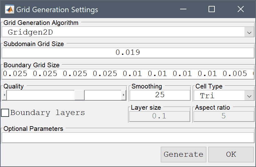
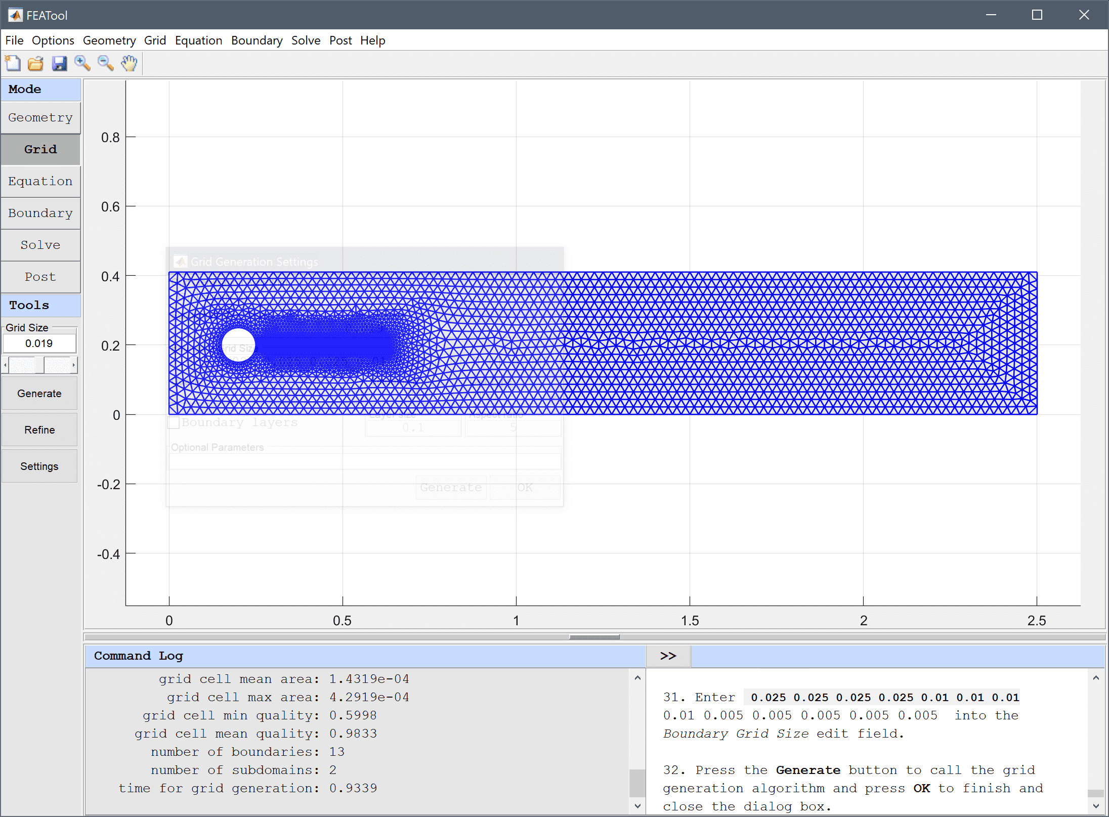
Press the Generate button to call the grid generation algorithm and press OK to finish and close the dialog box.
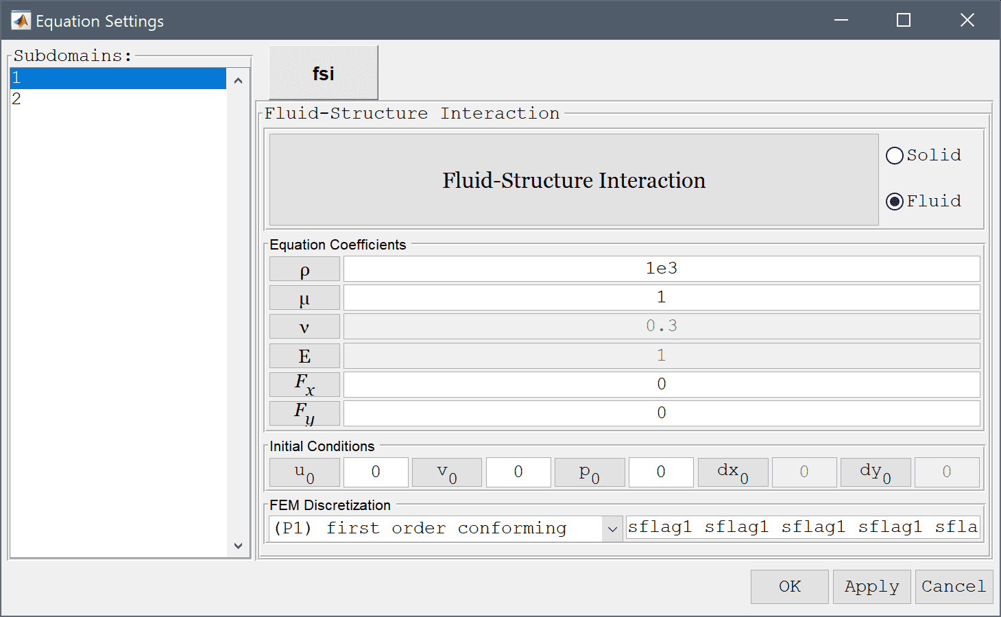
In the Equation Settings dialog box that automatically opens, select the fluid domain, 1 in the Subdomains list box, and set the density ρ to 1e3 and viscosity µ to 1 in the corresponding edit fields. The other coefficients can be left to their default values.
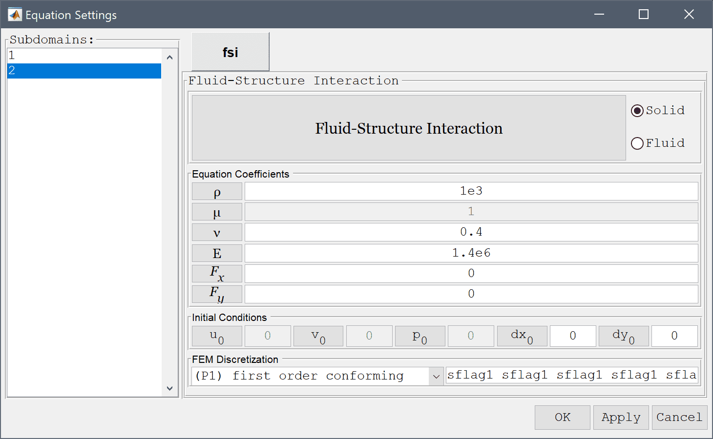
Set the density ρ to 1e3, Poisson's ratio ν to 0.4, and modulus of elasticity E to 1.4e6. Then press OK to finish and close the dialog box.
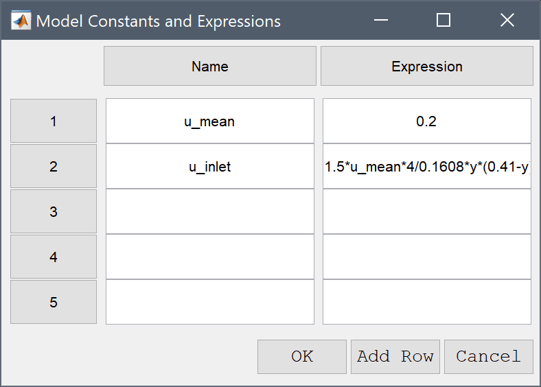
Press the Constants Toolbar button, or select the corresponding entry from the Equation menu, to open the Model Constants and Expressions dialog box. Enter a constant value of 0.2 for the mean velocity u_mean. Also enter the expression 1.5*u_mean*4/0.1608*y*(0.41-y)*(0.5*(1-cos(pi/2*t))*(t<2)+(t>=2)) for the inlet velocity u_in. This expression defines a parabolic inlet profile 1.5*u_mean*4/0.1608*y*(0.41-y) which is successively applied between t = 0-2 by using the scaling factor (0.5*(1-cos(pi/2*t))*(t<2)+(t>=2)).
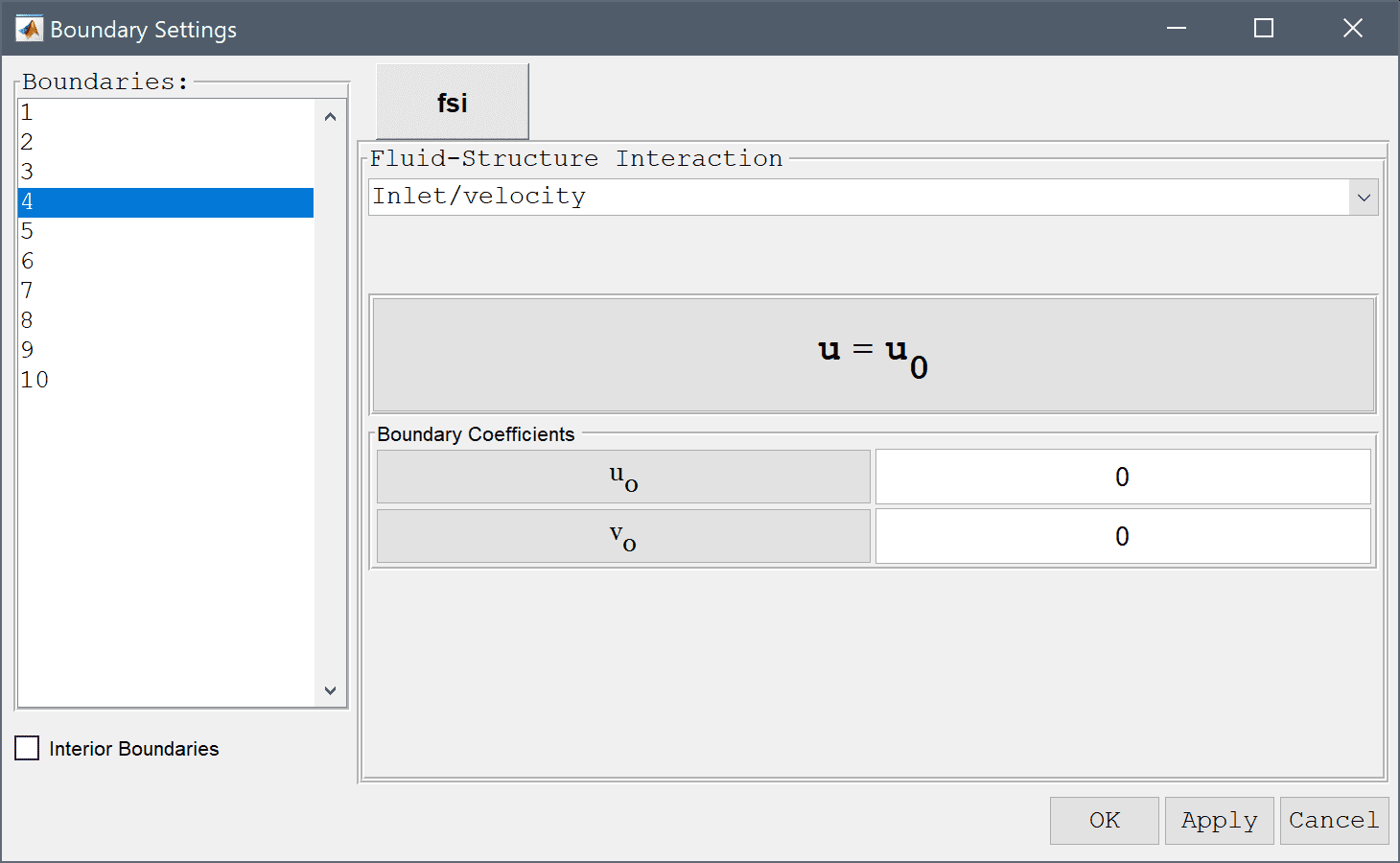
First select the left inflow boundary (number 4) and choose the Inlet/velocity boundary condition from the drop-down menu. Enter u_inlet in the edit field for the velocity coefficient in the x-direction to use the pre-defined expression for the inlet velocity.
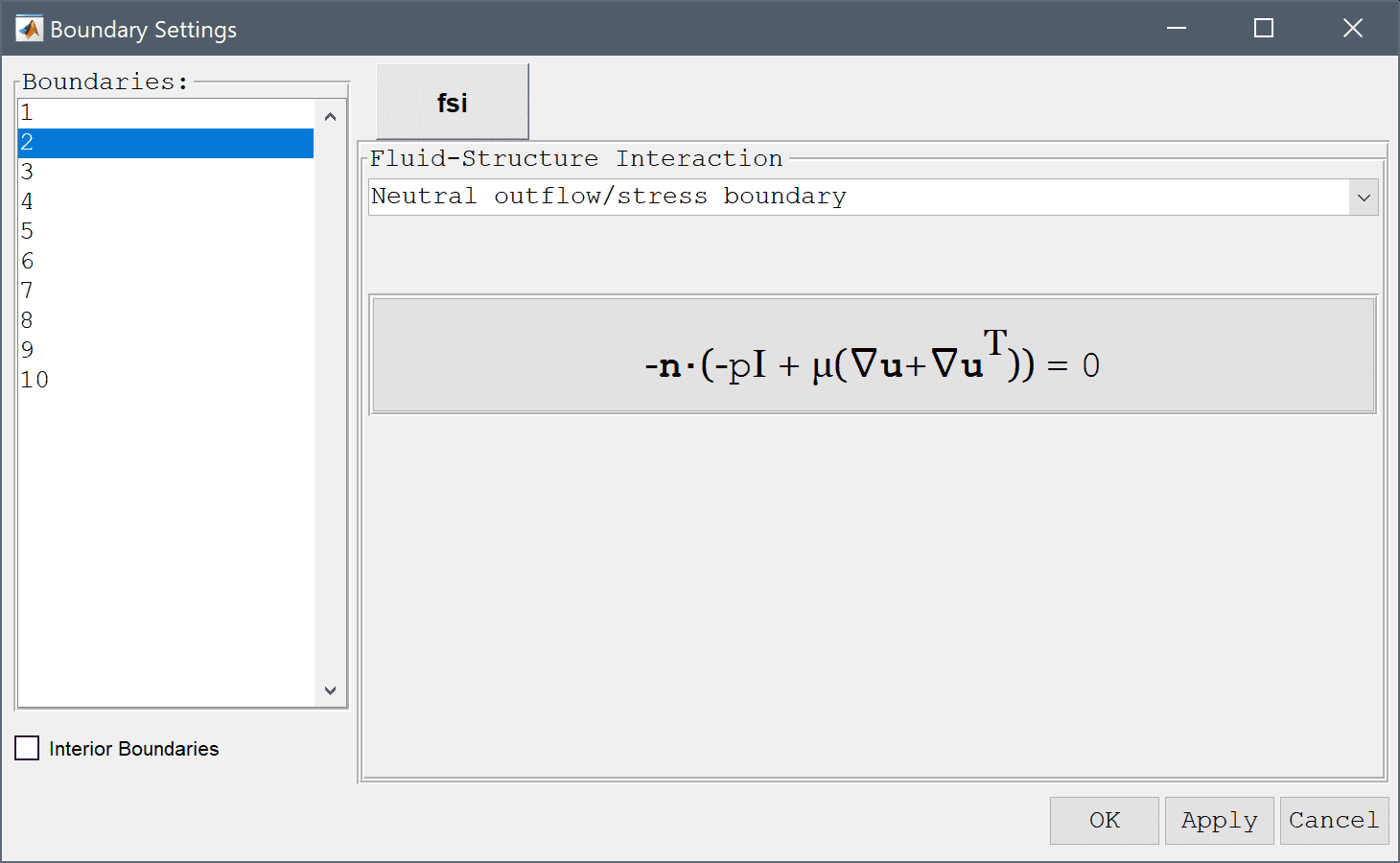
Select the right outflow boundary (number 2) and select the Neutral outflow/stress boundary boundary condition from the drop-down menu.
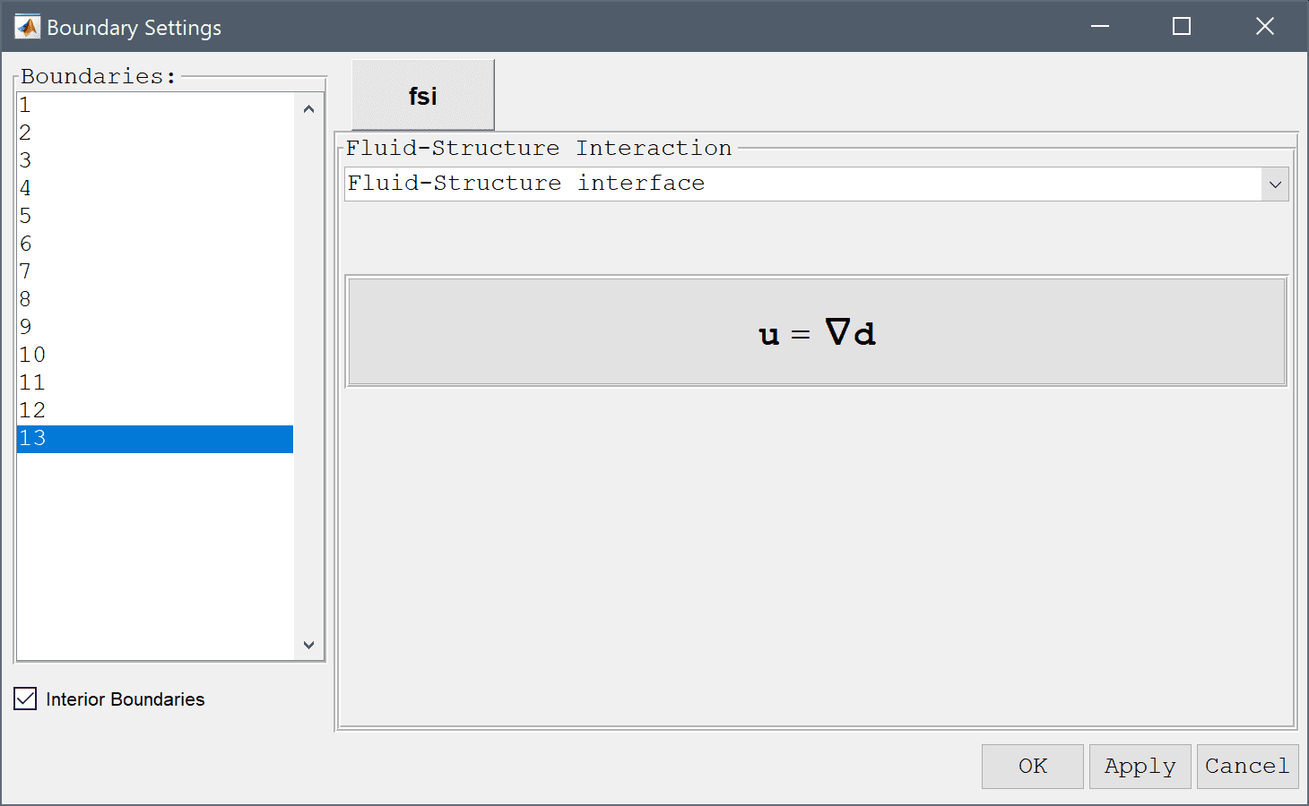
Select the Fluid-Structure interface condition for the boundaries shared between the fluid and solid (11, 12, and 13).
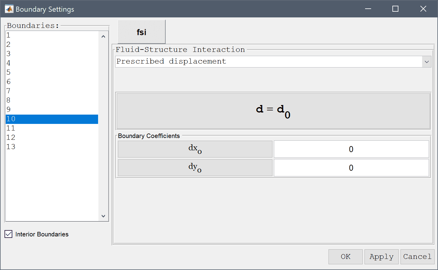
Finally, select the Prescribed displacement boundary condition with zero displacement to fix the right edge of the beam (boundaries 9 and 10). Then press OK to finish the boundary condition specification
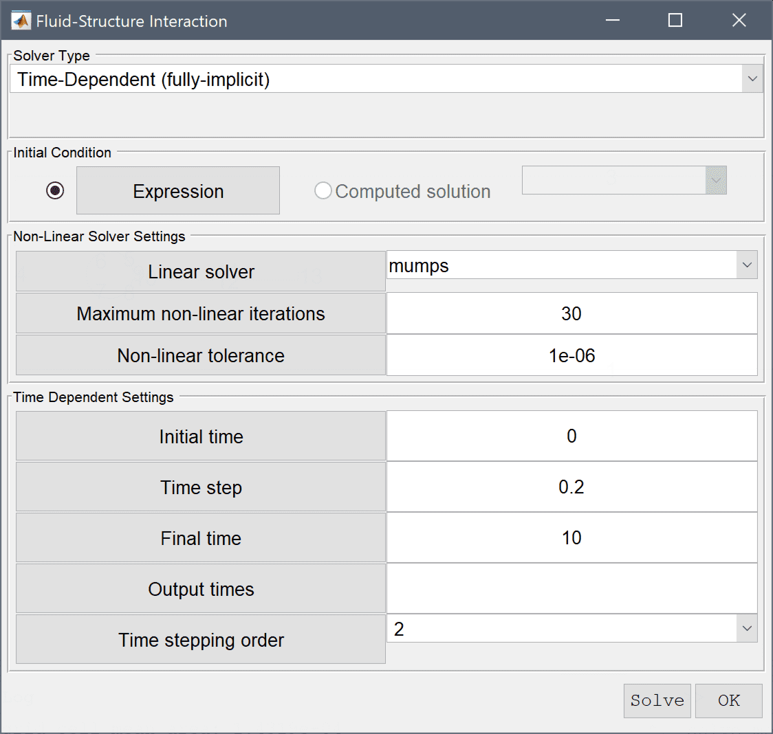
Set the time step to 0.2 and final time to 10 which should give enough time to develop a steady solution. Then press Solve to start the solution process.
Press the Solve button.
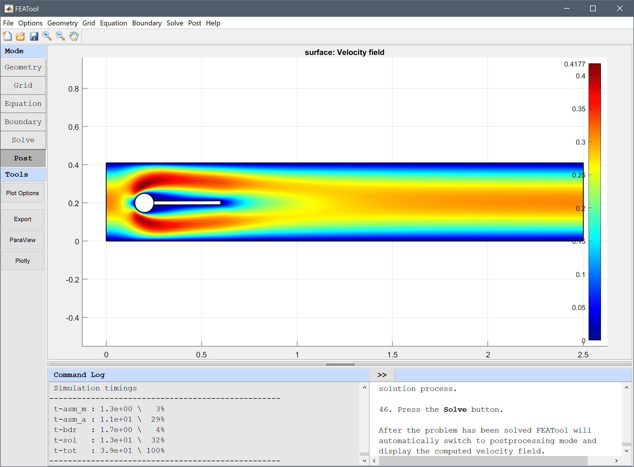
After the problem has been solved FEATool will automatically switch to postprocessing mode and display the computed velocity field.
To calculate the drag and lift forces, first select Boundary Integration... from the Post menu. In the Boundary Integration dialog box, select the boundaries which make up the circle and beam in the left hand side Boundaries selection list box (numbers 5-8 and 11-13). Then select the corresponding Total force, x-component from the pre-defined integration expressions. Press the OK or the Apply button to show the result in the lower Integration Result frame as well as in the Command Log message window.
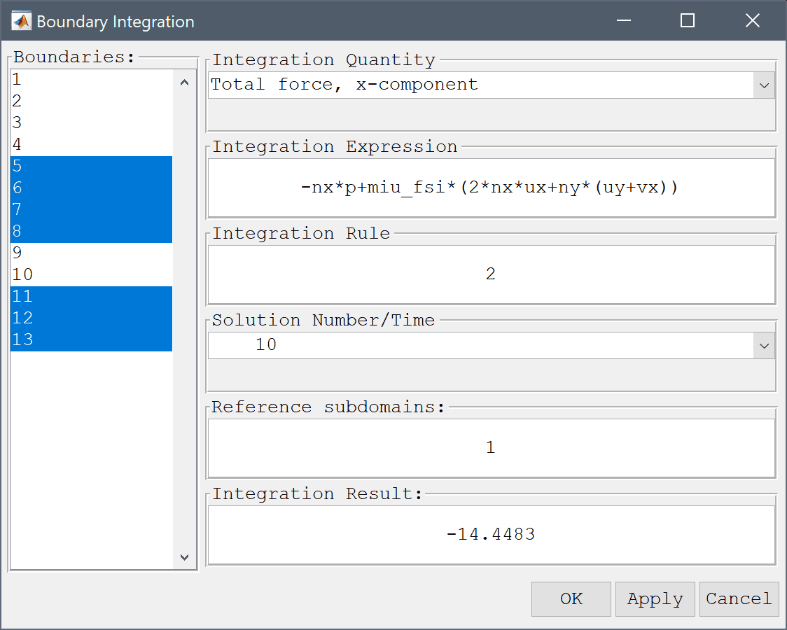
The computed drag force is about 14.4483 which is close to the reference value of 14.29426. Now repair the process for the force in the y-direction.
Similarly, the computed lift force is about 0.81534 in the y-direction which should be compared to the reference value of 0.763746. To get a closer result one could use a finer grid along the cylinder and beam boundaries, as well as higher order elements which yield higher accuracy for quantities involving derivatives (as the force terms here do)
To set an instationary test case, go back and increase the density of the beam to 1e4 and change the mean inlet velocity to 1. Also decrease the time step of the solver to 0.01 and the final time to 15. Note that, depending on your system configuration, the instationary simulation may take a long time to finish.

The fluid-structure interaction - elastic beam multiphysics model has now been completed and can be saved as a binary (.fea) model file, or exported as a programmable MATLAB m-script text file (available as the example ex_fluidstructure1 script file), or GUI script (.fes) file.
[1] Hron J. A monolithic FEM/multigrid solver for ALE formulation of fluid structure interaction with application in biomechanics. In H.-J. Bungartz and M. Schaefer, editors, Fluid-Structure Interaction: Modelling, Simulation, Optimisation, LLNCSE. Springer, 2006.