Stress Distribution in a Solenoid

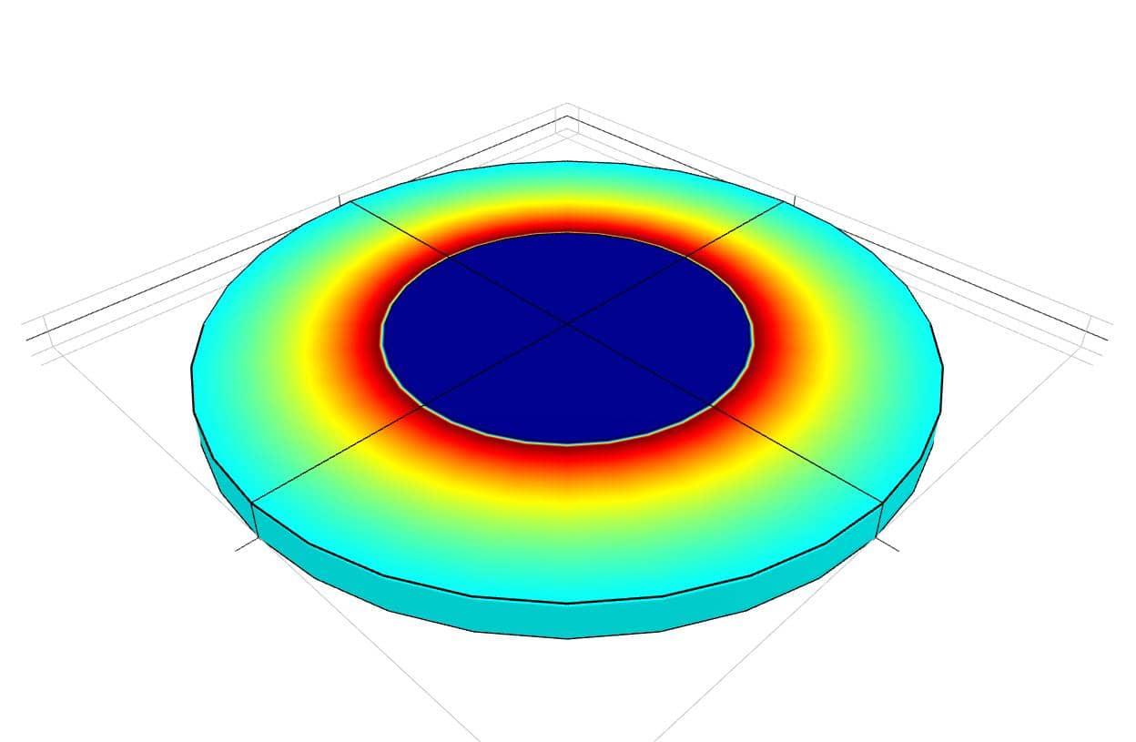
This multiphysics model examines how magnetic forces give rise to stresses in a long thick cylindrical solenoid. A current density of 10⁶ A/m² is running through a wound coil with 1 cm inner to 2 cm outer radii. The material of the coil is assumed to have a modulus of elasticity of 1.075⋅10¹¹ N/m² and Poisson's ratio of 0.33, and air occupies the inner hollow core.

As this is a one-way coupled problem, the magnetostatic effects will be solved for first, after which the calculated magnetic forces will be used as input to the stress-strain problem. Due to symmetry it is also sufficient to model a 2D axisymmetric cross-section. The resulting magnetic flux density and circumferential stress at r = 1.3 cm will be compared to the theoretical values of 8.798⋅10^-3 T and 96.71 N/m, respectively [1].

Tutorial

This model is available as an automated tutorial by selecting Model Examples and Tutorials... > Multiphysics > Stress Distribution in a Solenoid from the File menu. Or alternatively, follow the step-by-step instructions below.

1. To start a new model click the New Model toolbar button, or select New Model... from the File menu.
2. Select the Axisymmetry radio button.

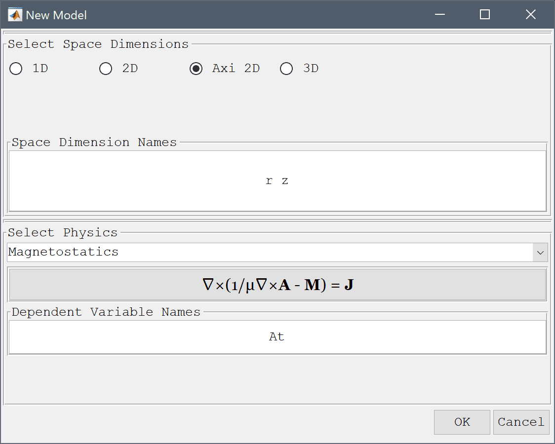
3. Select the Magnetostatics physics mode from the Select Physics drop-down menu.

   
4. Press OK to finish the physics mode selection.

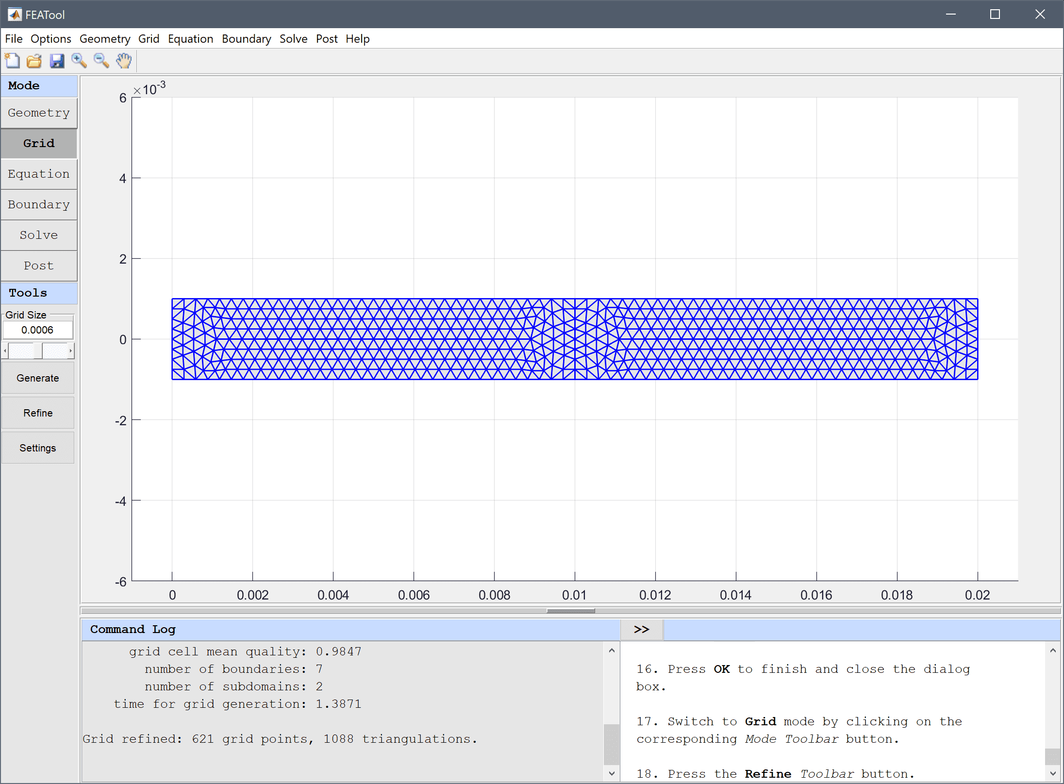
The geometry here consists of two rectangular subdomains the inner air r = 0-1 cm and the solenoid r = 1-2 cm, as the solution is expected to be symmetric in the axial direction the height does not influence the solution.

1. Select Rectangle from the Geometry menu.
2. Enter 0 into the x_min edit field.
3. Enter 1e-2 into the x_max edit field.
4. Enter -1e-3 into the y_min edit field.

5. Enter 1e-3 into the y_max edit field.

   
6. Press OK to finish and close the dialog box.
7. Select Rectangle from the Geometry menu.
8. Enter 1e-2 into the x_min edit field.
9. Enter 2e-2 into the x_max edit field.
10. Enter -1e-3 into the y_min edit field.
11. Enter 1e-3 into the y_max edit field.

12. Press OK to finish and close the dialog box.

    
13. Switch to Grid mode by clicking on the corresponding Mode Toolbar button.
14. Press the Refine Toolbar button.
15. Switch to Equation mode by clicking on the corresponding Mode Toolbar button.

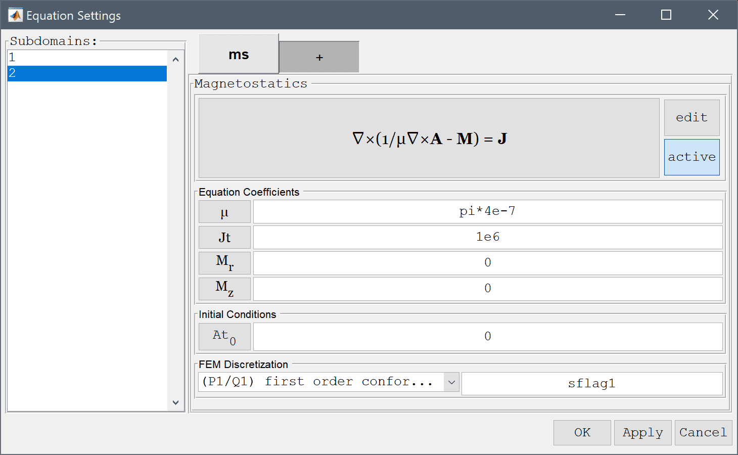
Equation and material coefficients can be specified in Equation/Subdomain mode. In the Equation Settings dialog box that automatically opens, enter a current density of 10⁶ A/m² for the second subdomain. The other coefficients can be left to their default values.

Note that FEATool works with any unit system, and it is up to the user to use consistent units for geometry dimensions, material, equation, and boundary coefficients.

1. Select 1 in the Subdomains list box.
2. Enter 0 into the Current density, θ edit field.
3. Select 2 in the Subdomains list box.

4. Enter 1e6 into the Current density, θ edit field.

   
5. Switch to the + tab.

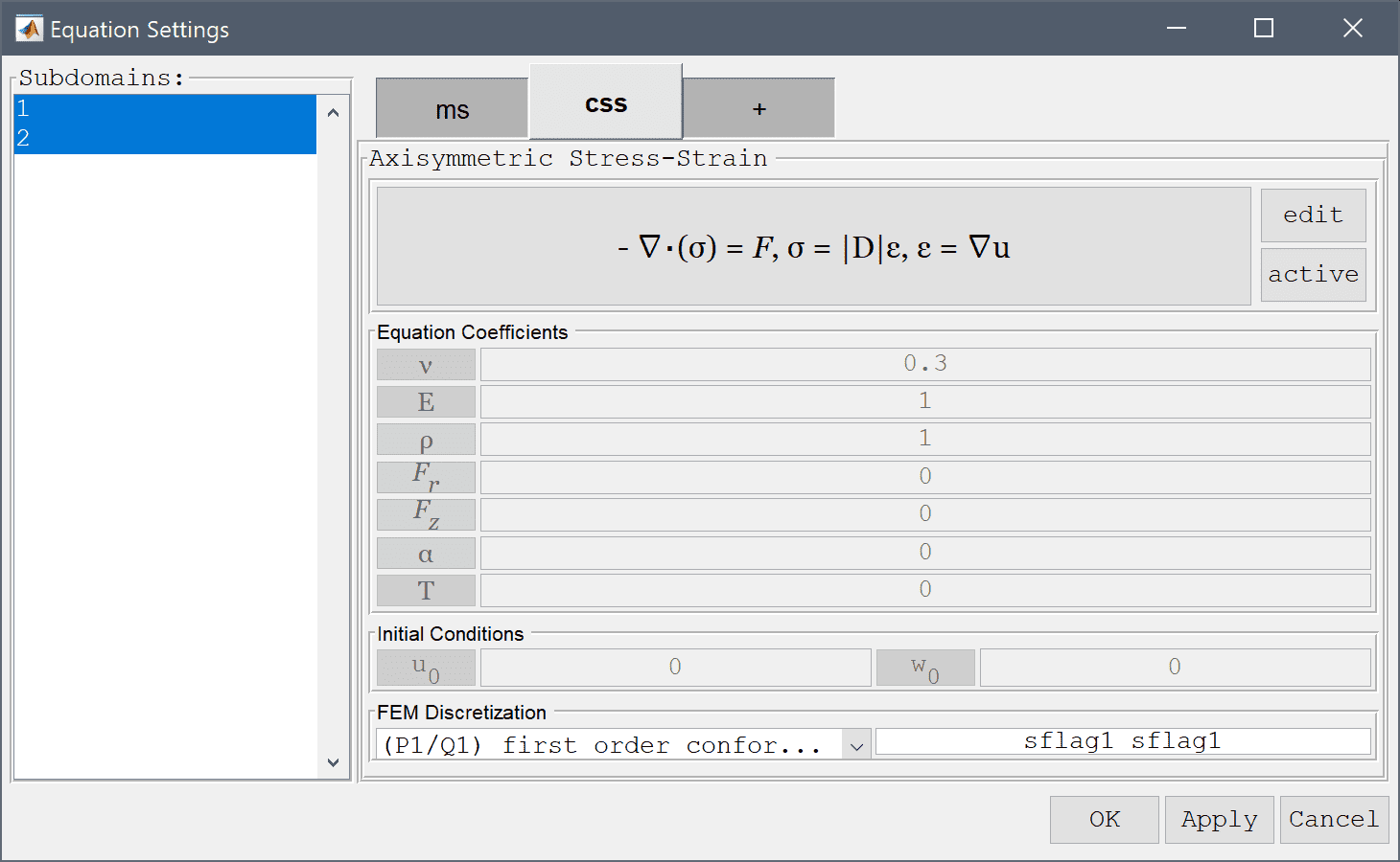
We will add a axisymmetric stress-strain inactive physics mode, to be used in the second solution step.

1. Select the Axisymmetric Stress-Strain physics mode from the Select Physics drop-down menu.
2. Press the Add Physics >>> button.
3. Switch to the css tab.
4. Select 1 and 2 in the Subdomains list box.

5. Press the active toggle button.

   
6. Press OK to finish the equation and subdomain settings specification.
7. Switch to Boundary mode by clicking on the corresponding Mode Toolbar button.
8. Select 1, 2, 4, 5, and 6 in the Boundaries list box.

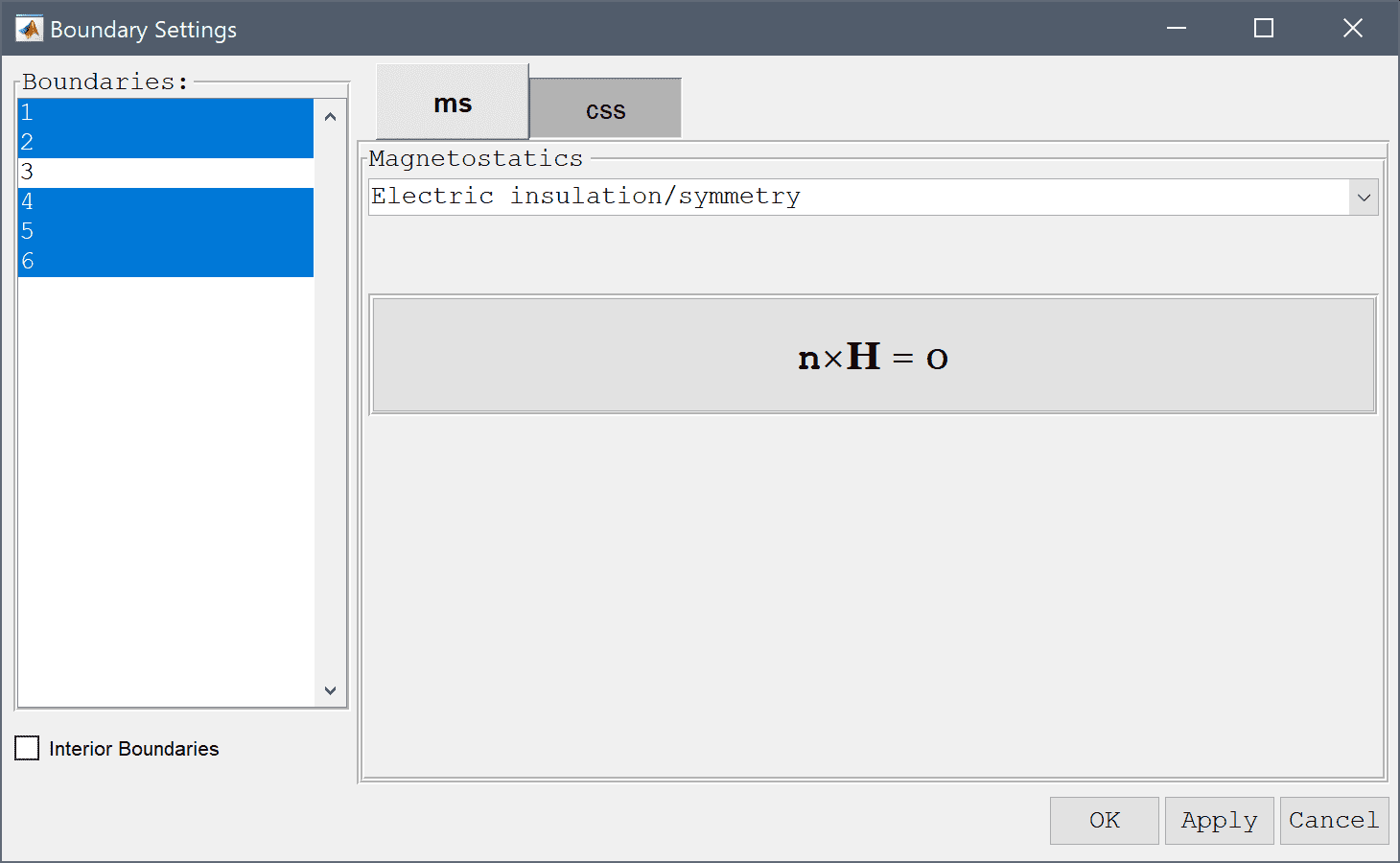
9. Select Electric insulation/symmetry from the Magnetostatics drop-down menu.

   

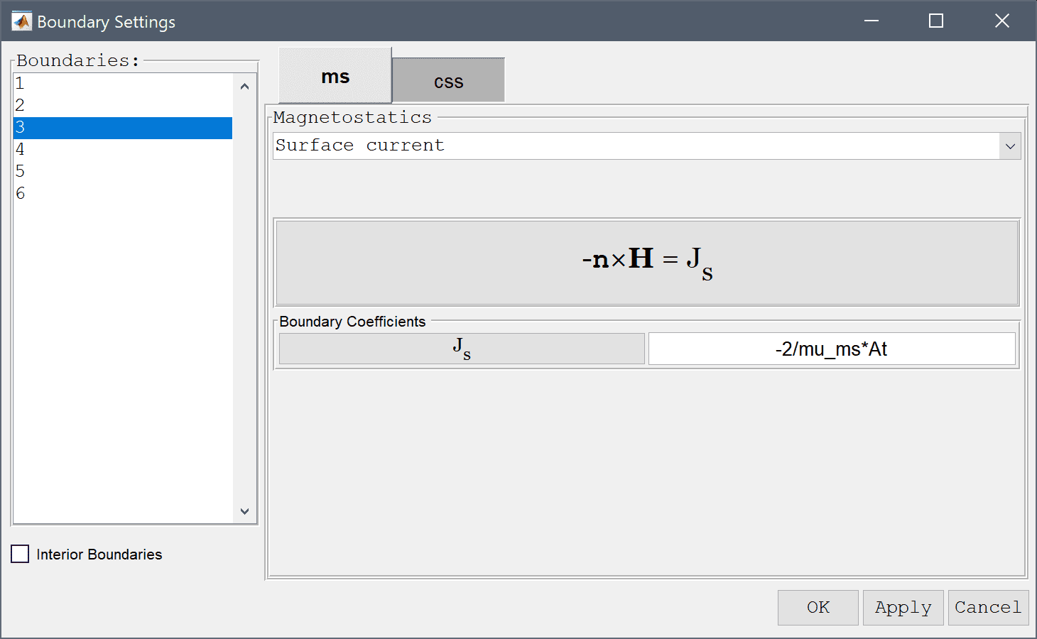
Select the inner boundary and modify the surface current/Neumann boundary coefficient to -2/mu_ms*At in order to manually prescribe a neutral axis Robin boundary condition.

1. Select 3 in the Boundaries list box.
2. Select Surface current from the Magnetostatics drop-down menu.

3. Enter -2/mu_ms*At into the Surface current edit field.

   
4. Press OK to finish the boundary condition specification.
5. Now that the problem is fully specified, press the Solve Mode Toolbar button to switch to solve mode. Then press the = Tool button to call the solver with the default solver settings.

After the problem has been solved FEATool will automatically switch to postprocessing mode and here display the computed magnetic potential. To change the plot, open the postprocessing settings dialog box by clicking on the Plot Options Toolbar button.

1. Press the Plot Options Toolbar button.
2. Select Magnetic flux density from the Predefined surface plot expressions drop-down menu.
3. Select the Contour Plot check box.
4. Select Magnetic flux density from the Predefined contour plot expressions drop-down menu.
5. Enter 25 into the Number or specified vector of contour levels to plot edit field.

6. Press OK to plot and visualize the selected postprocessing options.

   

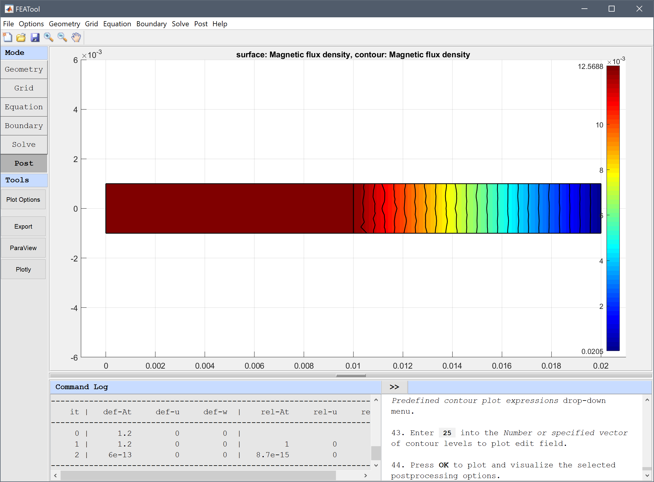
Using the point evaluation tool we can evaluate the flux density to compare with the expected value.

1. Select Point/Line Evaluation... from the Post menu.
2. Select Magnetic flux density, z-direction from the Evaluation Expression drop-down menu.
3. Enter 0.013 into the Evaluation coordinates in r-direction edit field.
4. Enter 0 into the Evaluation coordinates in z-direction edit field.

5. Press the Apply button.

   

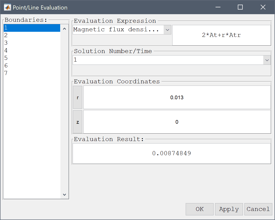
A computed flux density of 8.749e-3 T compares well with the expected value of 8.798e-3 T.

1. Press OK to finish and close the dialog box.

Now in the second step we go back and deactivate the magnetostatics physics mode and activate and solve for the stress-stain. Although we could solve both physics simultaneously, since the model only features a one way coupling, magnetic forces to stress-strain, we can save computational time and cost by solving in two steps.

1. Switch to Equation mode by clicking on the corresponding Mode Toolbar button.
2. Select 1 and 2 in the Subdomains list box.
3. Press the active toggle button.
4. Switch to the css tab.
5. Select 2 in the Subdomains list box.
6. Press the active toggle button.
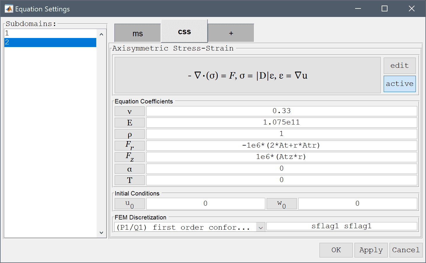
7. Enter 0.33 into the Poisson's ratio edit field.
8. Enter 1.075e11 into the Modulus of elasticity edit field.

The resulting magnetic body forces are here due to the product of the current density and B field.

1. Enter -1e6*(2*At+r*Atr) into the Body load in r-direction edit field.

2. Enter 1e6*(Atz*r) into the Body load in z-direction edit field.

   
3. Press OK to finish the equation and subdomain settings specification.

Due to symmetry the z-displacement is fixed at the top and bottom boundaries.

1. Switch to Boundary mode by clicking on the corresponding Mode Toolbar button.
2. Switch to the css tab.
3. Select 4 and 6 in the Boundaries list box.
4. Select the Fixed displacement, w radio button.
5. Press OK to finish the boundary condition specification.
6. Switch to Solve mode by clicking on the corresponding Mode Toolbar button.

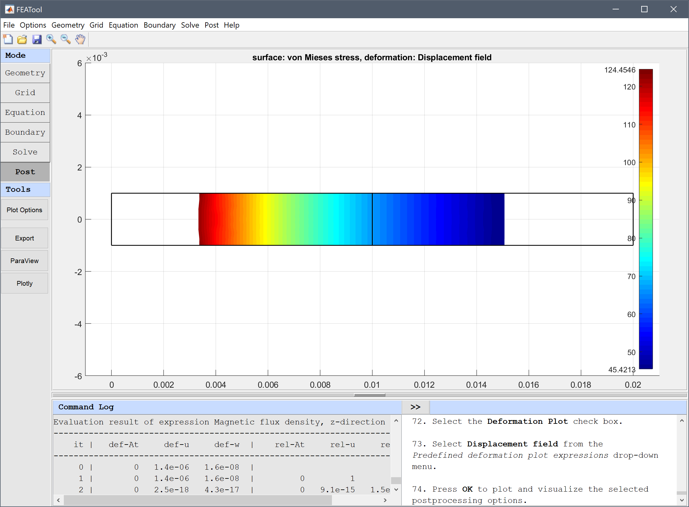
Note that the restart button is used here instead of the solve button = in order to use the existing already computed solution for the magnetic field.

1. Press the Solve with last computed solution as initial condition Toolbar button.
2. Press the Plot Options Toolbar button.
3. Select von Mieses stress from the Predefined surface plot expressions drop-down menu.
4. Clear the Contour Plot check box.
5. Select the Deformation Plot check box.
6. Select Displacement field from the Predefined deformation plot expressions drop-down menu.

7. Press OK to plot and visualize the selected postprocessing options.

   
8. Select Point/Line Evaluation... from the Post menu.
9. Select Stress, theta-component from the Evaluation Expression drop-down menu.
10. Enter 0.013 into the Evaluation coordinates in r-direction edit field.
11. Enter 0 into the Evaluation coordinates in z-direction edit field.

12. Press the Apply button.

    

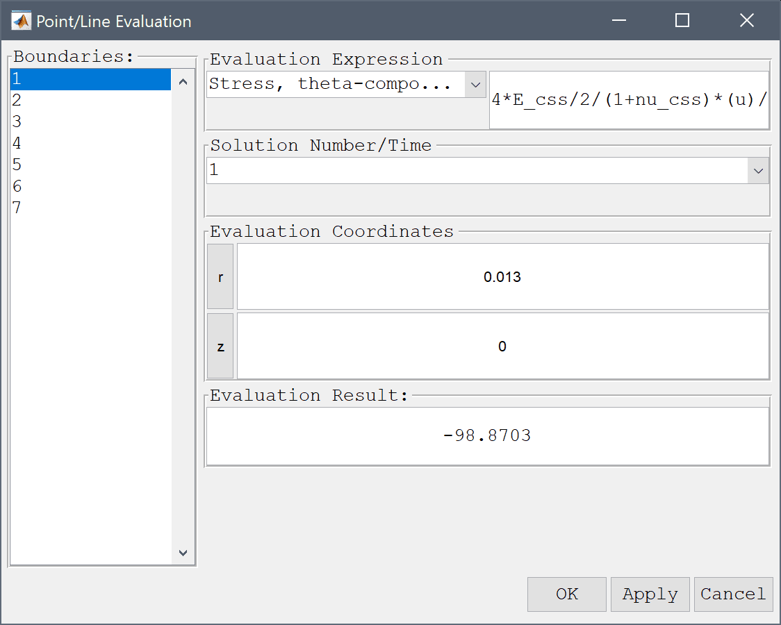
The computed angular stress of 98.87 N/m also compares well with the expected value of 96.71 N/m.

1. Press OK to finish and close the dialog box.

The stress distribution in a solenoid multiphysics model has now been completed and can be saved as a binary (.fea) model file, or exported as a programmable MATLAB m-script text file, or GUI script (.fes) file.

References

[1] Moon FA. Magneto-Solid Mechanics, Chapter 4, John Wiley & Sons, NY, 1984.