Electro-Osmotic Flow

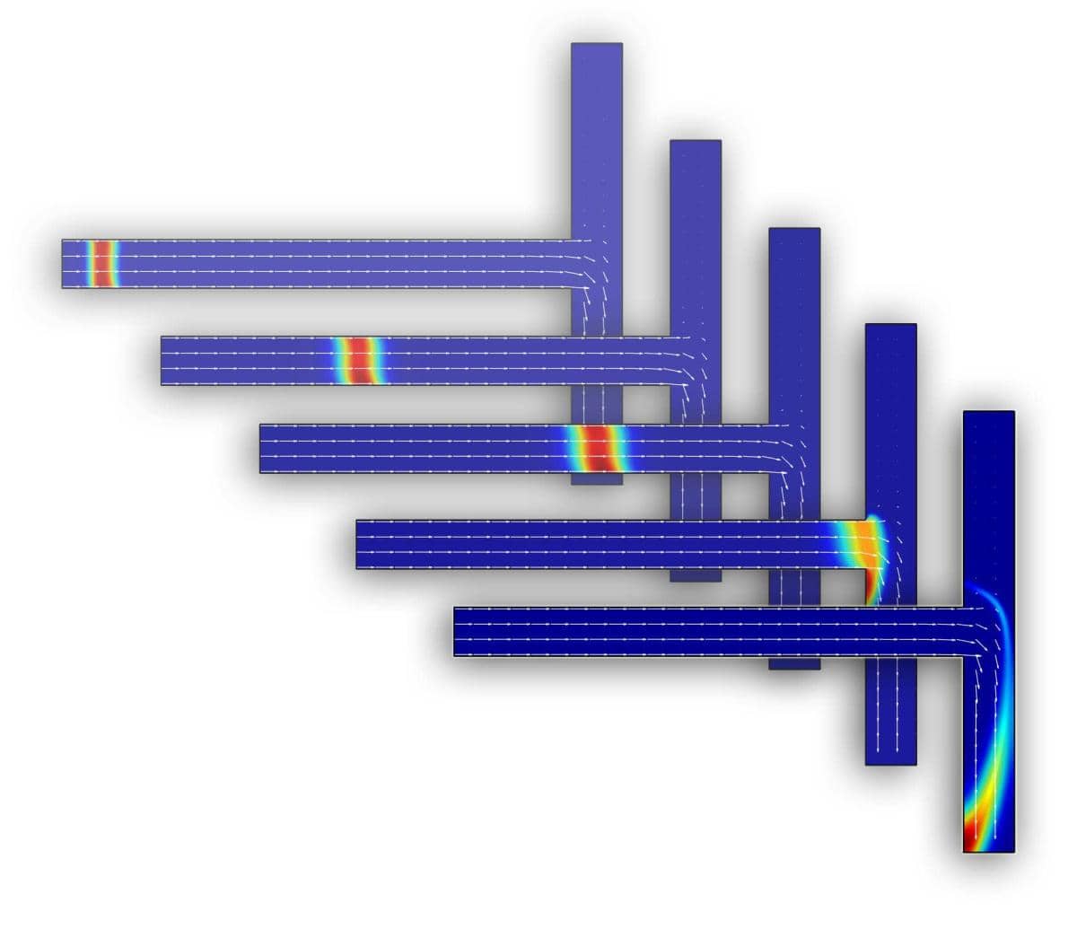
This multiphysics example examines microfluidic flow and coupled mass transport due to electroosmosis in a channel with a T-shaped junction. With application of an electric field in a micro channel a flow effect is induced along the walls due to chemical reactions between the liquid and the wall material. This effect is called electro-osmotic flow (EOF), and can for example be used in chemical analysis to separate reactants and chemical species. The flow effect is here modeled with the Helmholtz-Smoluchowski boundary condition [1,2] which prescribes a tangential slip velocity as

u_t = μ_EOF·E_t = μ_EOF·(E - (E·n)n)

where μ_EOF = εε₀ζ/μ is the electroosmotic mobility. In this model, the walls are aligned with the coordinate axes, and the boundary condition can therefore be simplified to -μ_EOFV_x and -μ_EOFV_y for the horizontal and vertical boundaries, respectively (where V_x and V_y are the gradients of the electric potential V). A passive scalar representing a chemical analyte is injected at the inlet for a prescribed duration (concentration 1 for t <= 30 and linearly decreasing for the next 10 µs) whereby the transport, diffusion, and path of the species is tracked through the channel.

Coupled electroosmotic flow and mass transport in a T-shaped junction

Tutorial

This model is available as an automated tutorial by selecting Model Examples and Tutorials... > Multiphysics > Electro-Osmotic Flow from the File menu. Or alternatively, follow the step-by-step instructions below.

1. To start a new model click the New Model toolbar button, or select New Model... from the File menu.

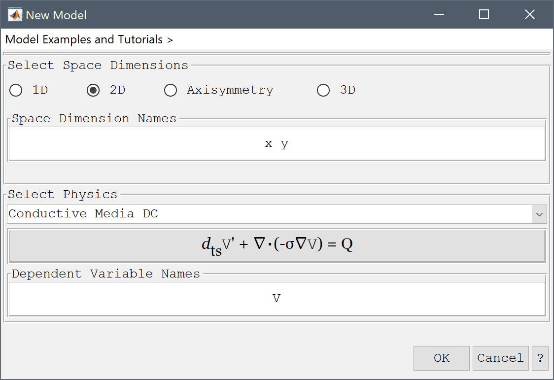
2. In the New Model dialog box, select 2D for the Space Dimensions, and select Conductive Media DC from the Select Physics drop-down menu (the physics modes for fluid flow and mass transport will be added later). Leave the space dimension and dependent variable names to their default values and press OK to finish the physics mode selection.

   

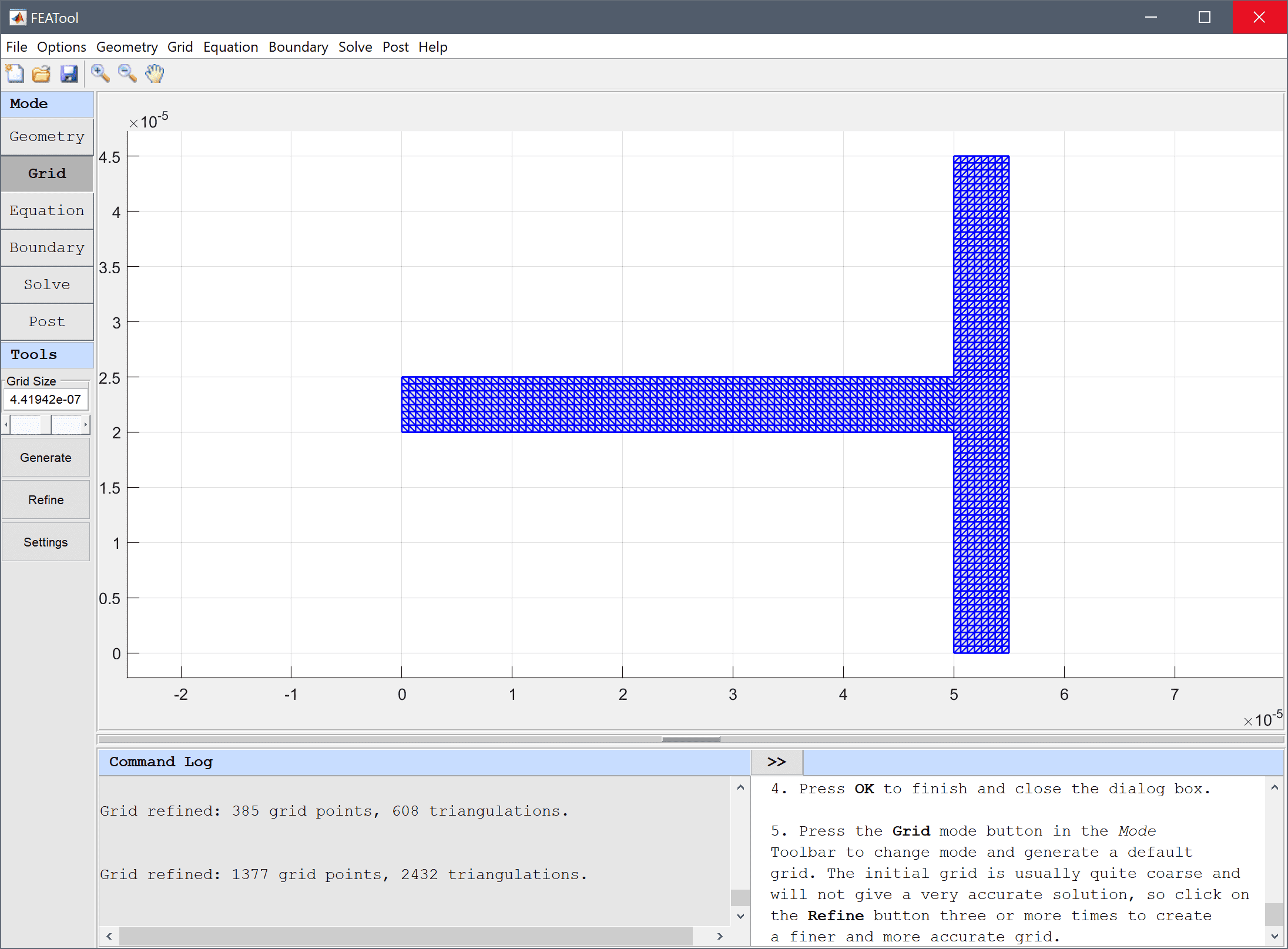
The geometry consists of a 45 by 55 micrometer T-shaped junction. One can either join two rectangles or use the polygon tool to create the shape of the geometry.

1. Select Polygon from the Geometry menu.

Enter the following data into the Point coordinates table.

	x	y
1	0	2e-05
2	5e-05	2e-05
3	5e-05	0
4	5.5e-05	0
5	5.5e-05	4.5e-05
6	5e-05	4.5e-05
7	5e-05	2.5e-05
8	0	2.5e-05

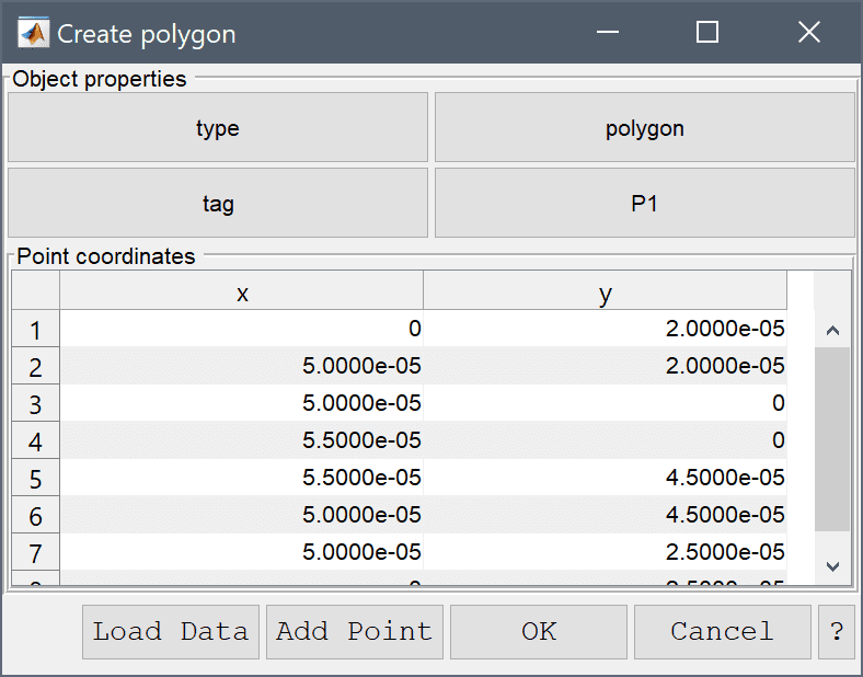
1. Press OK to finish and close the dialog box.

   

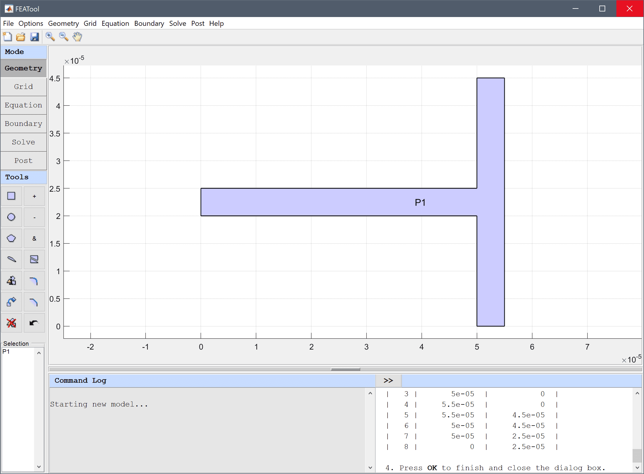
2. Press the Grid mode button in the Mode Toolbar to change mode and generate a default grid. The initial grid is usually quite coarse and will not give a very accurate solution, so click on the Refine button three or more times to create a finer and more accurate grid.

   
3. Press the Equation mode button to switch from grid mode to physics and equation/subdomain specification mode. Change to the + tab, in the Equation Settings dialog box that automatically opens, and add a Navier-Stokes physics mode for the fluid flow and Convection and Diffusion for the mass transport.
4. Switch to the + tab.
5. Select the Navier-Stokes Equations physics mode from the Select Physics drop-down menu.
6. Press the Add Physics >>> button.
7. Enter 1e3 into the Density edit field.
8. Enter 1e-3 into the Viscosity edit field.
9. Switch to the + tab.
10. Select the Convection and Diffusion physics mode from the Select Physics drop-down menu.
11. Press the Add Physics >>> button.

The species diffusion is assumed to be constant and small, while convection is due to the osmotic-velocity given by the Navier-Stokes physics mode (coupling u and v for the x and y-velocities, respectively).

1. Enter 1e-10 into the Diffusion coefficient edit field.
2. Enter u into the Convection velocity in x-direction edit field.

3. Enter v into the Convection velocity in y-direction edit field.

   

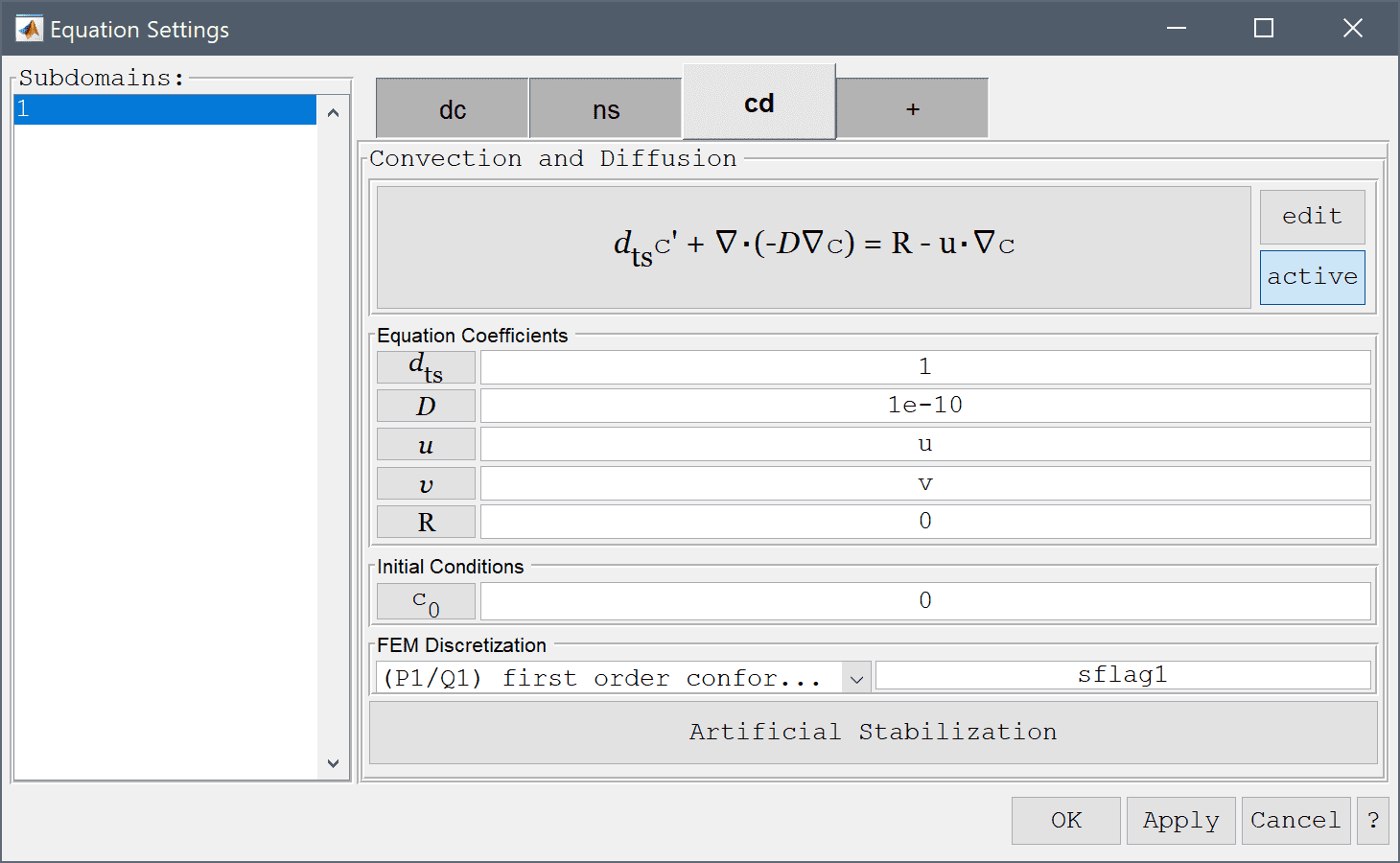
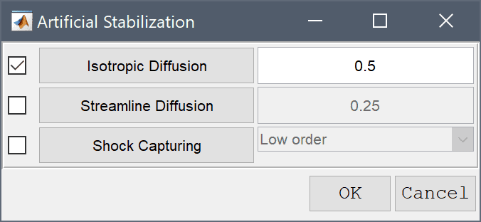
For convection dominated transport problems numerical diffusion can help to ensure a more physical and non-oscillatory solution. In this case isotropic diffusion is added (most diffusive), but more accurate streamline diffusion (less diffusive), or high order shock-capturing artificial diffusion can also be used, but are more costly and may take longer to compute a solution.

1. Press the Artificial Stabilization button.

2. Select the Check to enable isotropic artificial diffusion check box.

   
3. Press OK to finish and close the dialog box.
4. Press OK to finish the equation and subdomain settings specification.
5. Switch to Boundary mode by clicking on the corresponding Mode Toolbar button.

Boundary conditions are defined in Boundary Mode and describes how the model interacts with the surrounding environment.

The electric potential should be set to 100 V and the left side inlet, and 30 V and 0 at the top and bottom boundaries, respectively. Neutral current flow conditions are used for the walls.

1. First select all wall boundaries (here numbers 2, 4, 5, 7, and 8) in the Boundaries list box.
2. Select Current flow from the Conductive Media DC drop-down menu.
3. Select the left inlet, boundary 6.
4. Select Electric potential from the Conductive Media DC drop-down menu.
5. Enter 100 into the Electric potential edit field.
6. Select the top boundary 3.
7. Select Electric potential from the Conductive Media DC drop-down menu.
8. Enter 30 into the Electric potential edit field.
9. Select the bottom outlet boundary 1.
10. Select Electric potential from the Conductive Media DC drop-down menu.
11. Enter 0 into the Electric potential edit field.
12. Switch to the ns tab.

There should not be any forced flows or velocities prescribed, so first select Neutral conditions for all the inlets and outlets.

1. Select 1, 3, and 6 in the Boundaries list box.
2. Select Neutral outflow/stress boundary from the Navier-Stokes Equations drop-down menu.

Helmholtz-Smoluchowski boundary condition couples the electric field and gradient of the potential to the velocity at the walls and is driving the flow here. Since the walls are parallel to the coordinate axis the tangential component boundary conditions can be reduced to -5e-8*Vy and -5e-8*Vx in the x and y-directions.

1. Select 5 and 7 in the Boundaries list box.
2. Select Inlet/velocity from the Navier-Stokes Equations drop-down menu.

3. Enter -5e-8*Vx into the Velocity in x-direction edit field.

   
4. Select 2, 4, and 8 in the Boundaries list box.
5. Select Inlet/velocity from the Navier-Stokes Equations drop-down menu.
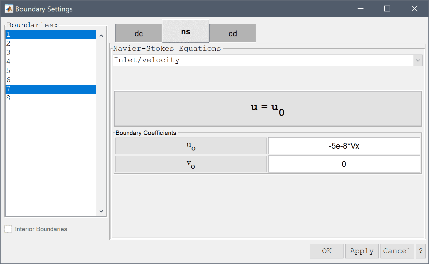
6. Enter -5e-8*Vy into the Velocity in y-direction edit field.

No species transport should be allowed through the walls and insulation conditions are therefore appropriate there.

1. Switch to the cd tab.
2. Select 2, 4, 5, 7, and 8 in the Boundaries list box.
3. Select Insulation/symmetry from the Convection and Diffusion drop-down menu.
4. Select 1 and 3 in the Boundaries list box.
5. Select Convective flux/outflow from the Convection and Diffusion drop-down menu.
6. Select 6 in the Boundaries list box.

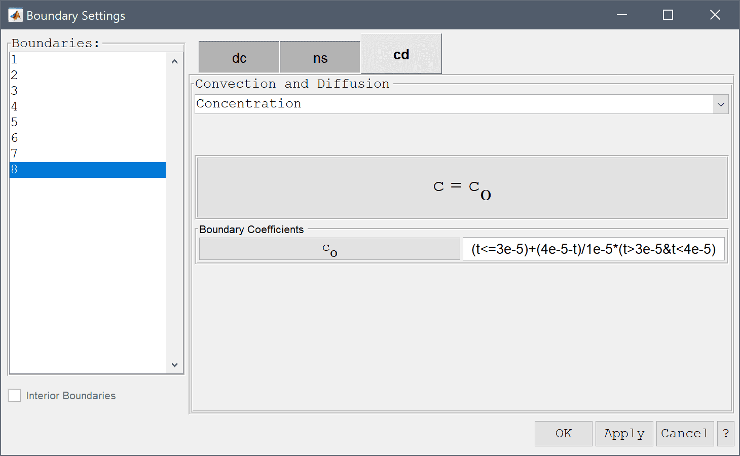
The inlet concentration should be 1 for t < 3e-5 and a linear decreasing function between 3e-5 < t < 4e-5. This can be represented as the switch condition (t<=3e-5)+(4e-5-t)/1e-5*(t>3e-5&t<4e-5) (where the logical conditions <, <=, and > either evaluate to zero or one.)

1. Select Concentration from the Convection and Diffusion drop-down menu.

2. Enter (t<=3e-5)+(4e-5-t)/1e-5*(t>3e-5&t<4e-5) into the Concentration edit field.

   
3. Press OK to finish the boundary condition specification.

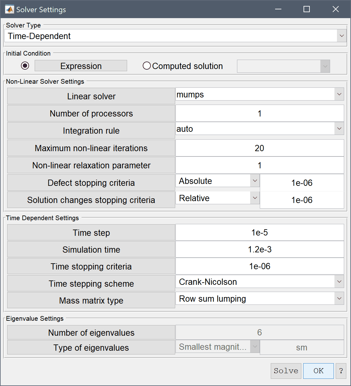
Now that the problem is fully specified, press the Solve Mode Toolbar button to switch to solve mode. Open the Solver Settings dialog box and select the time dependent solver, time step 1e-5 and simulation time 1.2e-3 seconds.

1. Switch to Solve mode by clicking on the corresponding Mode Toolbar button.
2. Press the Settings Toolbar button.
3. Select Time-Dependent from the Solution and solver type drop-down menu.
4. Enter 1e-5 into the Time step size edit field.

5. Enter 1.2e-3 into the Duration of time-dependent simulation (maximum time) edit field.

   

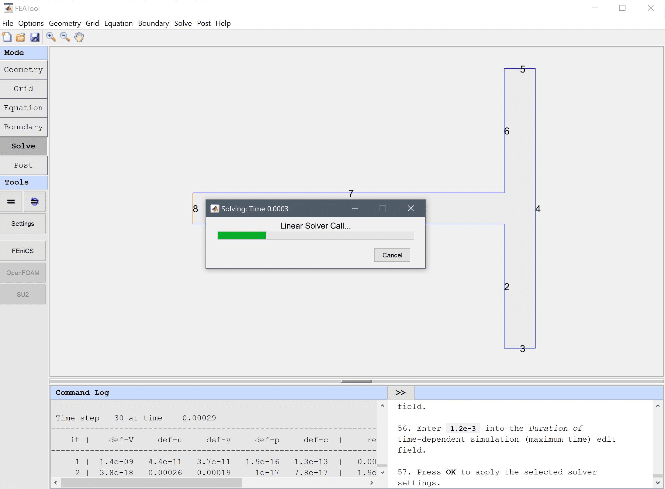
6. Press OK to apply the selected solver settings, and then press the = Toolbar button to call the solver.

   

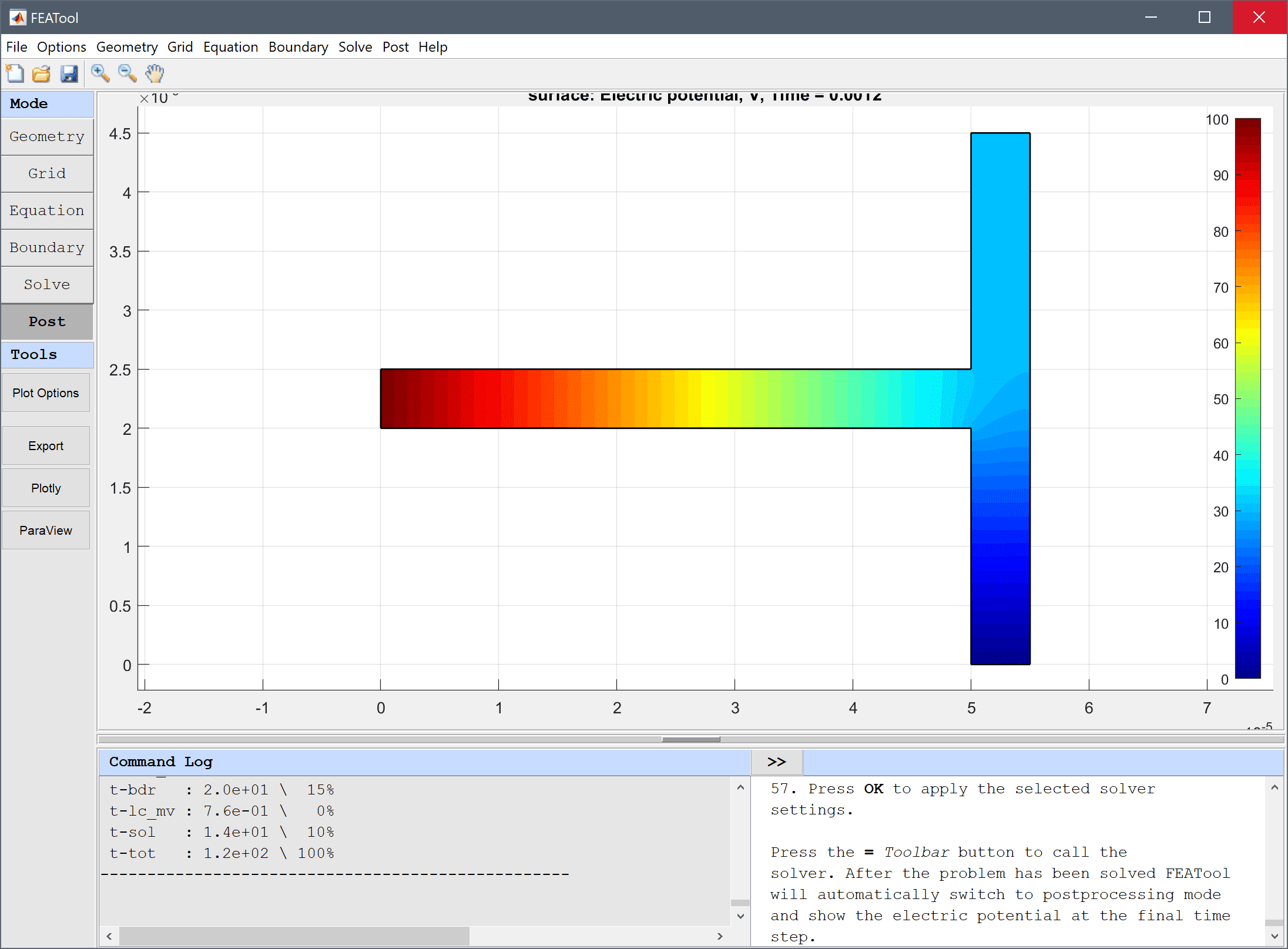
After the problem has been solved FEATool will automatically switch to postprocessing mode and show the electric potential at the final time step.

1. Press the Plot Options Toolbar button.

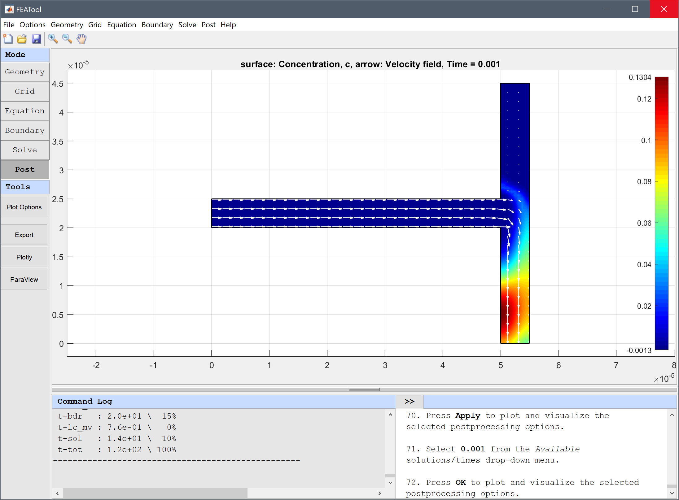
Also plot the velocity field to see how the majority of the flow takes the lower path.

1. Select Velocity field from the Predefined surface plot expressions drop-down menu.
2. Select the Enable/disable arrow plot check box.
3. Enter 30 into the Arrow spacing in y-direction (integer or coordinate vector) edit field.
4. Enter 30 into the Arrow spacing in x-direction (integer or coordinate vector) edit field.
5. Select white from the Select arrow color drop-down menu.
6. Select Velocity field from the Predefined arrow plot expressions drop-down menu.
7. Press Apply to plot and visualize the selected postprocessing options.

Finally plot the concentration at different times to see how the species is transported from the inlet to the outlet.

1. Select Concentration, c from the Predefined surface plot expressions drop-down menu.
2. Select 0.0001 from the Available solutions/times drop-down menu.
3. Press Apply to plot and visualize the selected postprocessing options.
4. Select 0.00075 from the Available solutions/times drop-down menu.
5. Press Apply to plot and visualize the selected postprocessing options.
6. Select 0.001 from the Available solutions/times drop-down menu.

7. Press OK to plot and visualize the selected postprocessing options.

   

To create an animation of the whole process one can use the Animate/Playback Solution... option from the Post menu.

Also note that in order to save computational resources it is possible to first compute stationary solutions for the electric potential and velocity field (as they will not change with time), and keep them constant (de-activated subdomains) while computing the mass transport problem (thus reducing the memory and time required for the time-dependent solver). See the Multi-Simulation Heat Exchanger for an example of this solution approach.

The electro-osmotic flow multiphysics model has now been completed and can be saved as a binary (.fea) model file, or exported as a programmable MATLAB m-script text file, or GUI script (.fes) file.

References

[1] G.E. Karniadakis and A. Beskok, Microflows: fundamentals and simulation. Springer-Verlag, New York, Berlin, Heidelberg, 2001.

[2] R.J. Yang, L.M. Fu, Y.C. Lin, Electroosmotic Flow in Microchannels. J. Colloid and Interface Science, 239:98-105, November 2001.