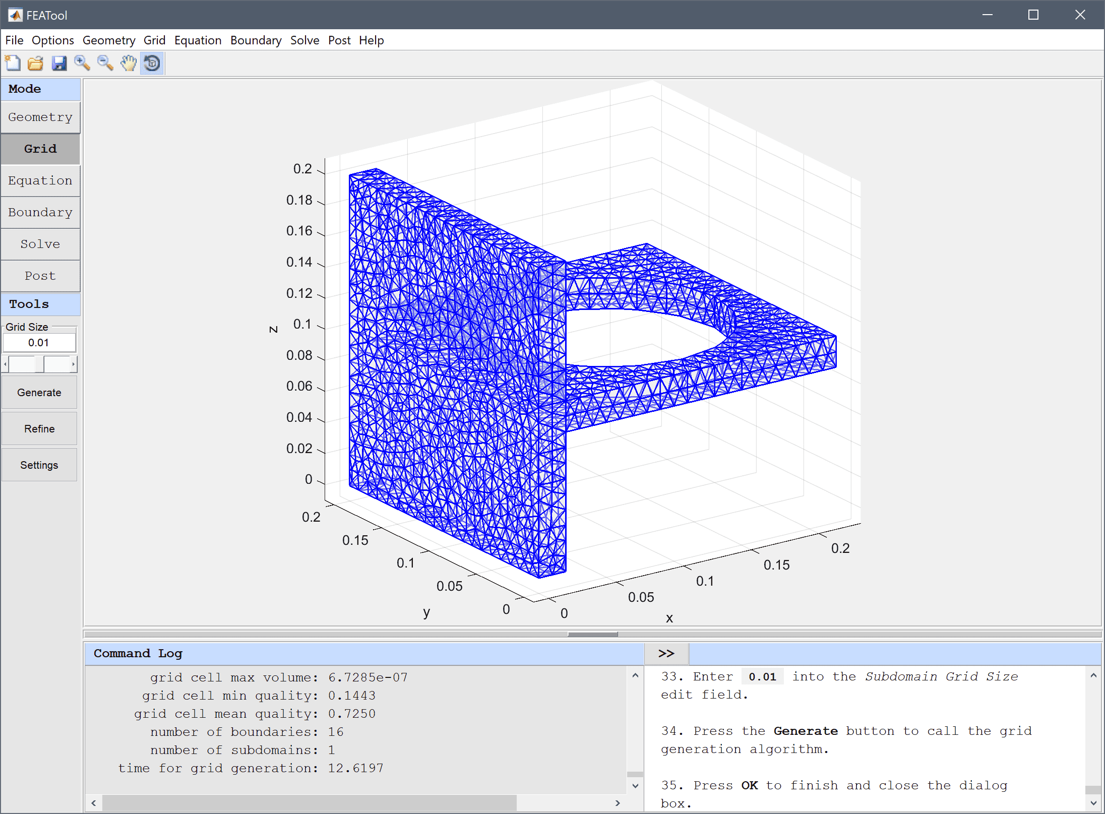
In this section a three dimensional model of a bracket with a hole will be described. The vertical side of the bracket is fixed to a wall (thus zero displacement boundary conditions are suitable here), while the outer end of the bracket is loaded with a negative force of -10000 N in the z-direction. The resulting displacements will be studied together with creating a displacement plot visualizing the deformation.

Tutorial

This model is available as an automated tutorial by selecting Model Examples and Tutorials... > Structural Mechanics > Deflection of a Bracket from the File menu. Or alternatively, follow the step-by-step instructions below.

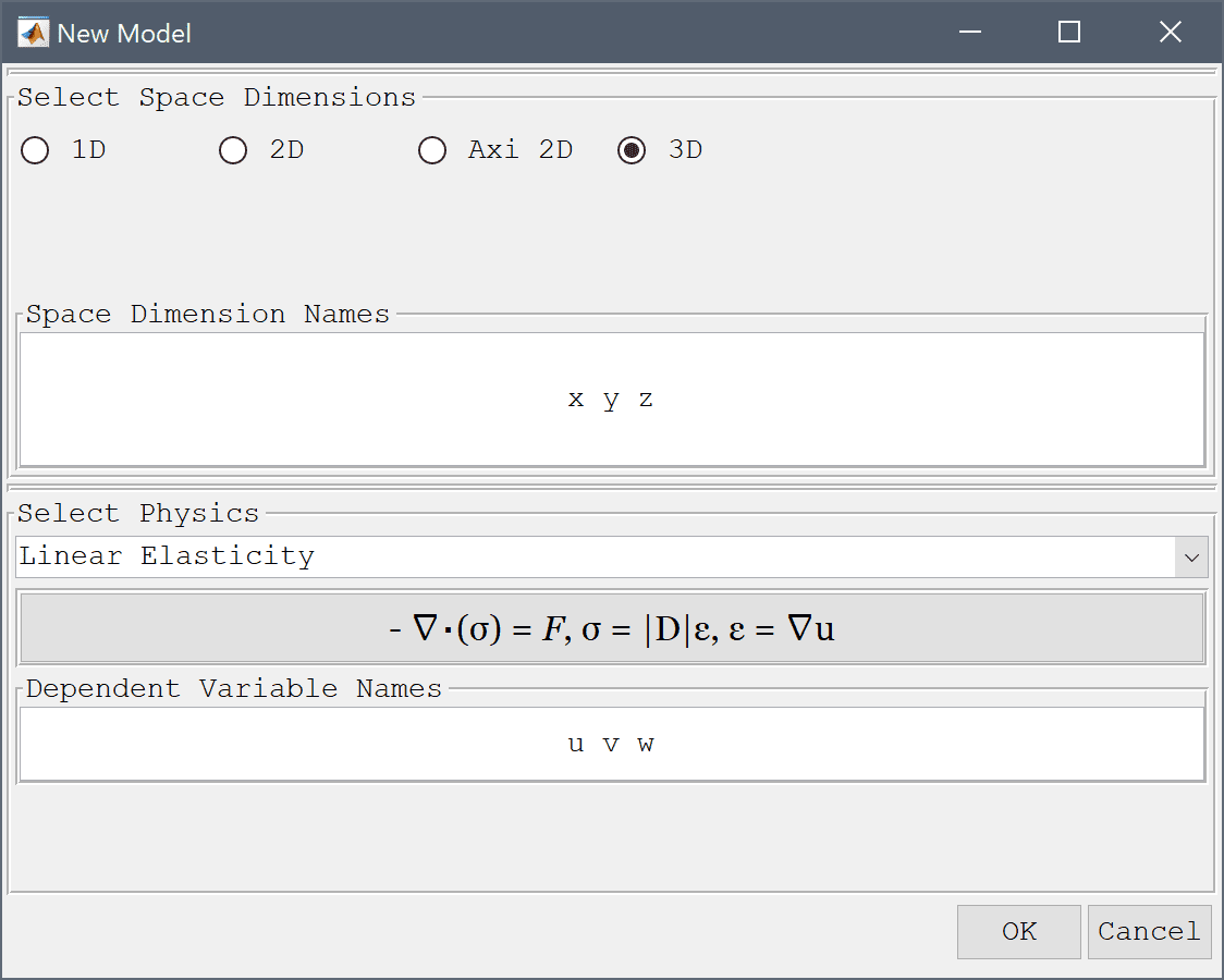
To start a new model click the New Model toolbar button, or select New Model... from the File menu.
Select the 3D radio button.
Select the Linear Elasticity physics mode from the Select Physics drop-down menu.
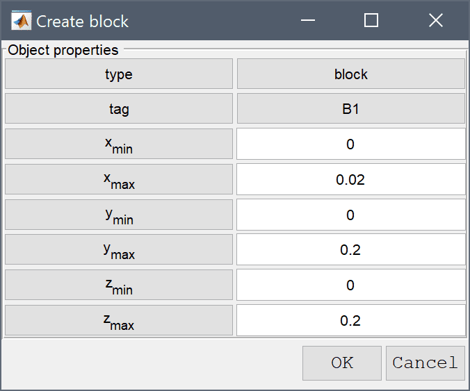
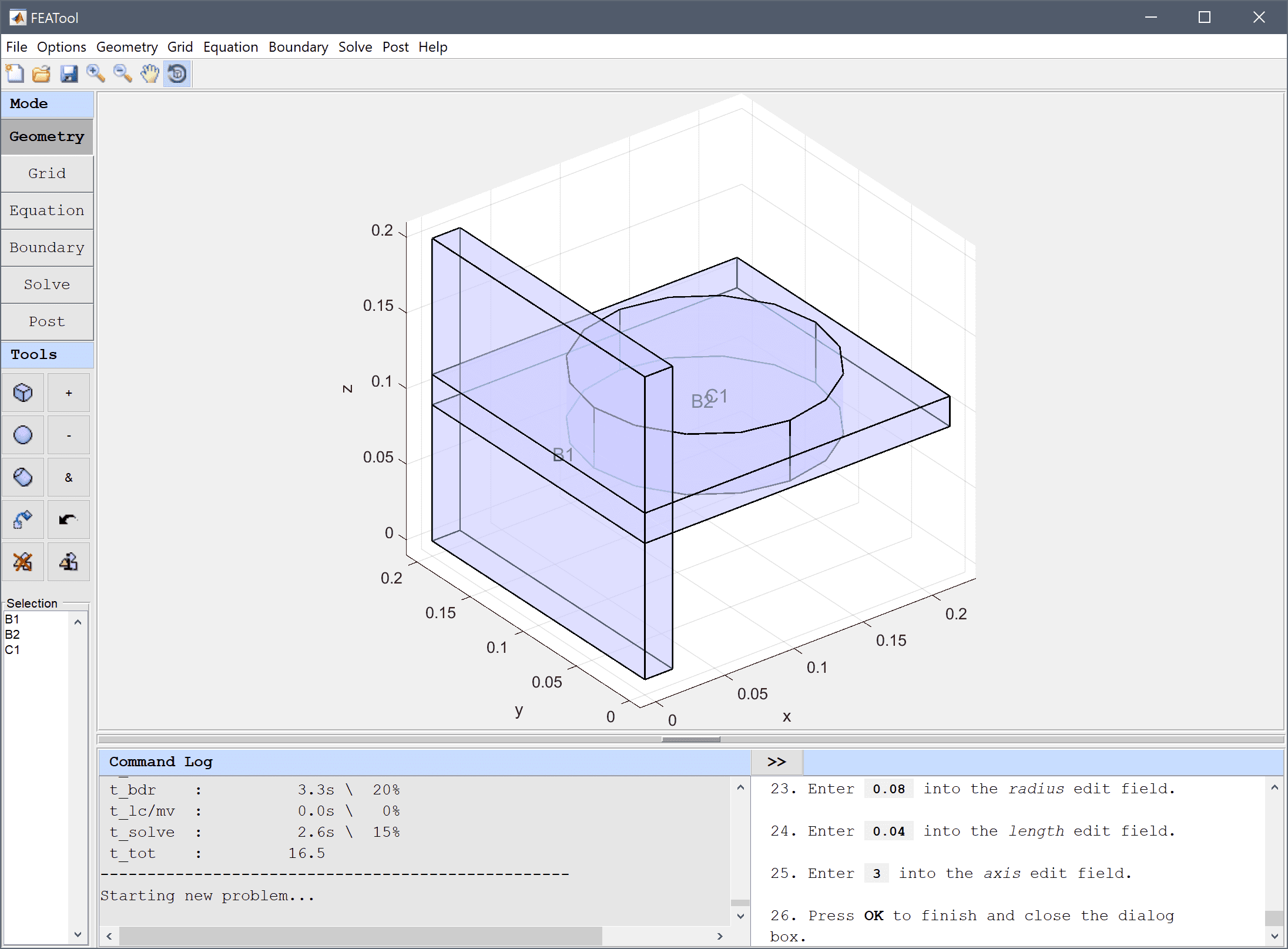
Press OK to finish the physics mode selection.

The geometry of the bracket can be made by combining two blocks and subtracting a cylinder for the hole.

Press the Create cube/block Toolbar button.
Enter 0 into the x_min edit field.
Enter 0.02 into the x_max edit field.
Enter 0 into the y_min edit field.
Enter 0.2 into the y_max edit field.
Enter 0 into the z_min edit field.
Enter 0.2 into the z_max edit field.
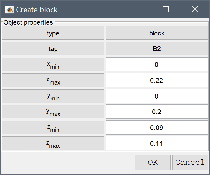
Press OK to finish and close the dialog box.
Press the Create cube/block Toolbar button.
Enter 0 into the x_min edit field.
Enter 0.22 into the x_max edit field.
Enter 0 into the y_min edit field.
Enter 0.2 into the y_max edit field.
Enter 0.09 into the z_min edit field.
Enter 0.11 into the z_max edit field.
Press OK to finish and close the dialog box.
Press the Create cylinder Toolbar button.
Enter 0.12 0.1 0.08 into the center edit field.
Enter 0.08 into the radius edit field.
Enter 0.04 into the length edit field.
Enter 3 into the axis edit field.
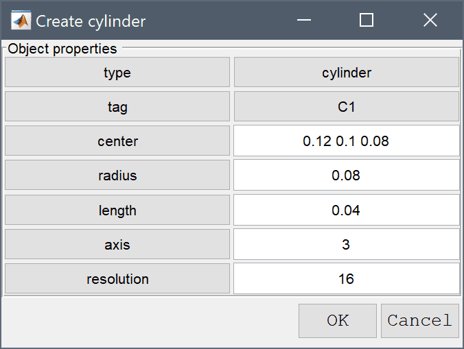
Press OK to finish and close the dialog box.
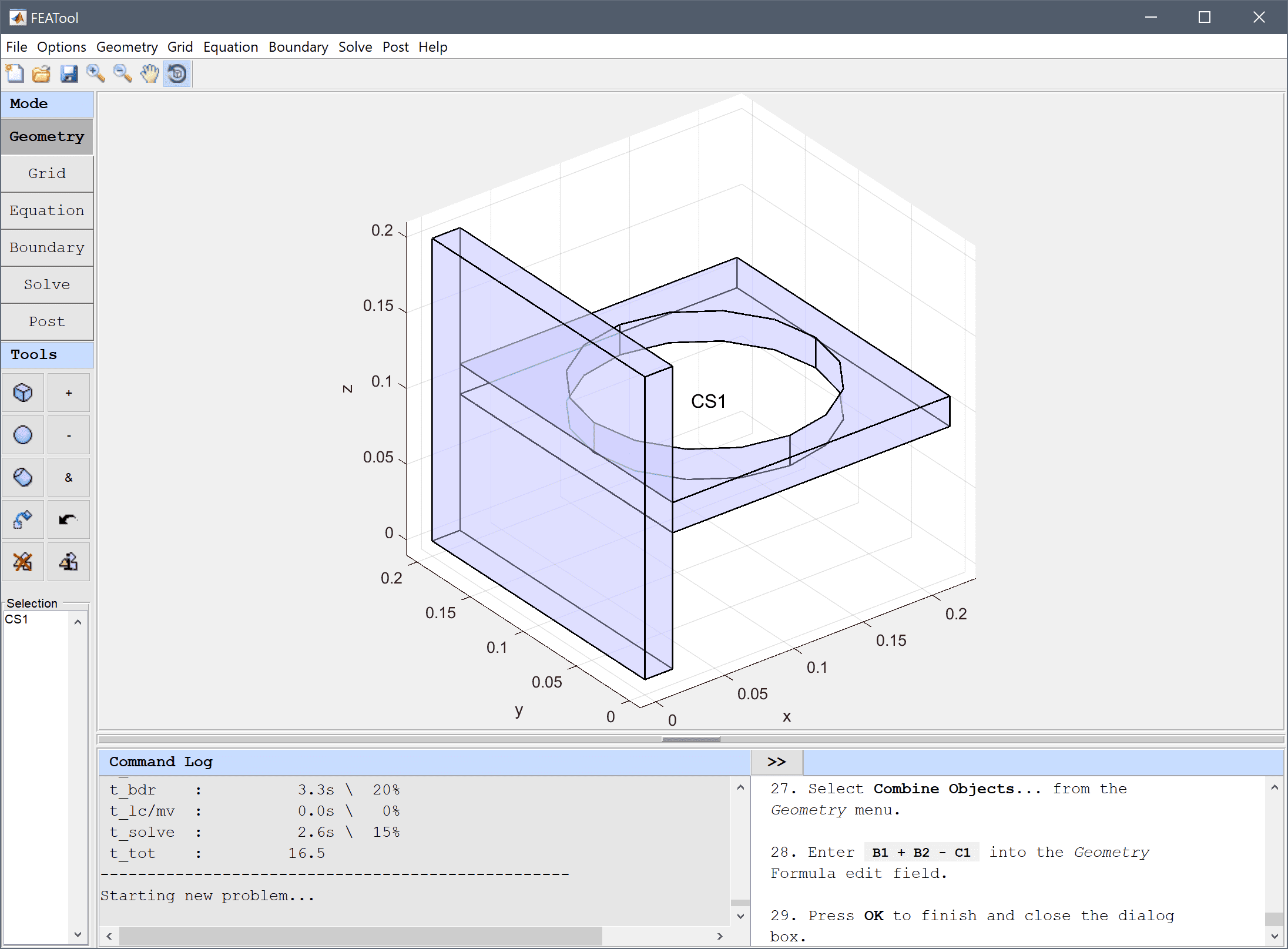
Select Combine Objects... from the Geometry menu.
Enter B1 + B2 - C1 into the Geometry Formula edit field.
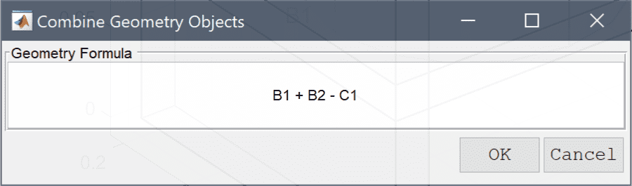
Press OK to finish and close the dialog box.
Switch to Grid mode by clicking on the corresponding Mode Toolbar button.
Press the Settings Toolbar button.
Enter 0.01 into the Subdomain Grid Size edit field.
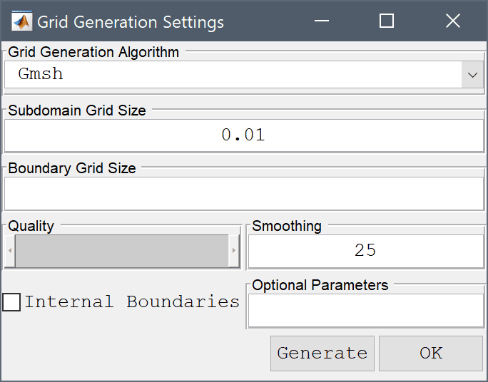
Press the Generate button to call the grid generation algorithm.
Press OK to finish and close the dialog box.
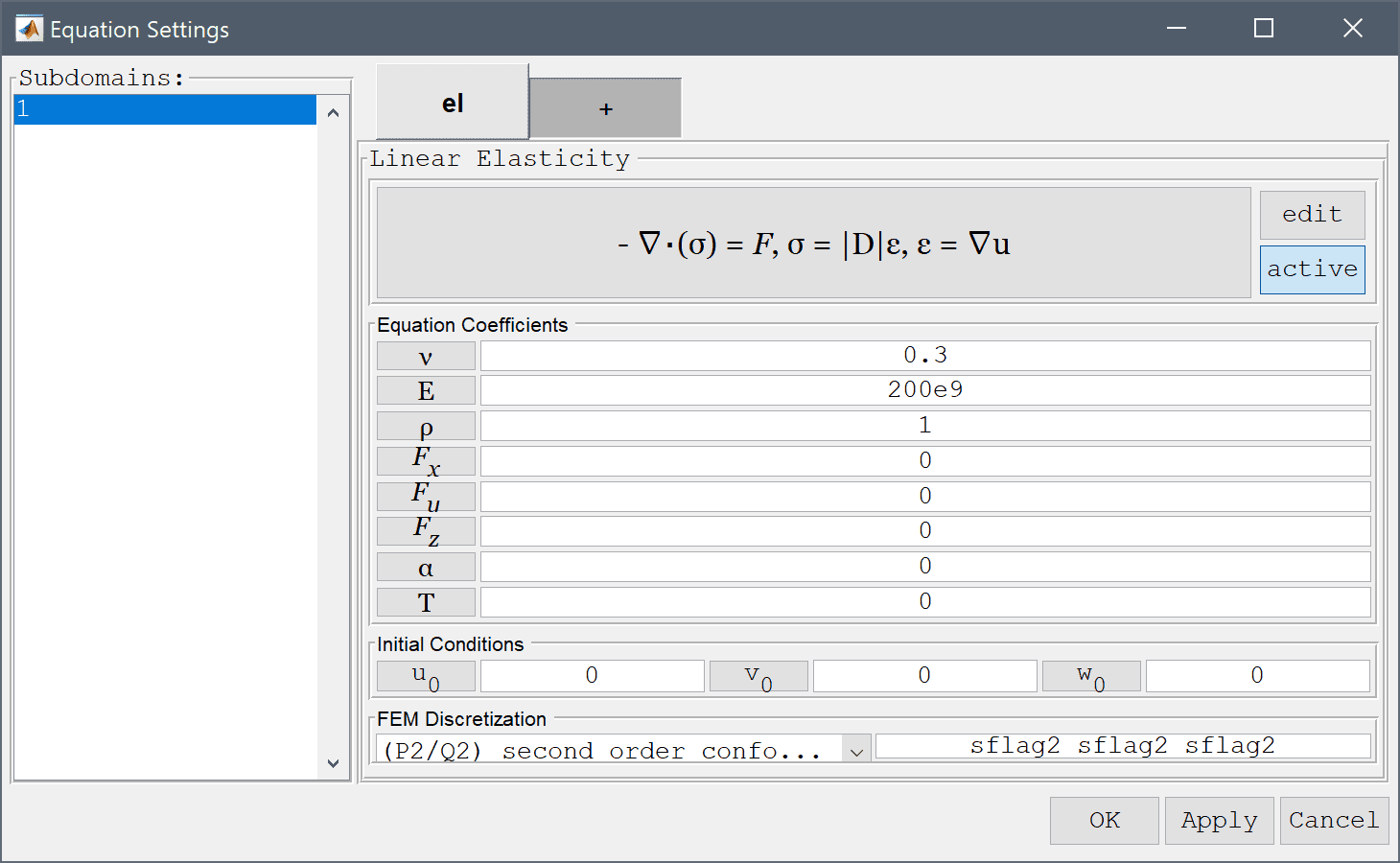
Switch to Equation mode by clicking on the corresponding Mode Toolbar button.
In the Equation Settings dialog box that automatically opens, set Poisson's ratio to 0.3 and the modulus of elasticity, E to 200e9 in the corresponding edit fields. The other coefficients can be left to their default values.
For more accurate solutions to expressions involving derivatives such as stresses choose a higher order finite element approximation, such as P2 second order FEM basis functions. Select (P2/Q2) second order conforming from the FEM Discretization drop-down menu, and press OK to finish and close the dialog box.
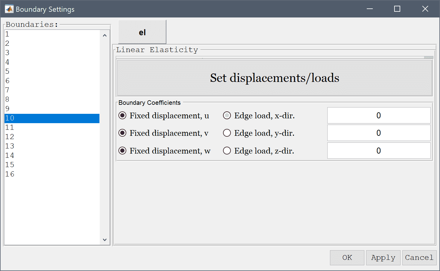
Switch to Boundary mode by clicking on the corresponding Mode Toolbar button.
In the Boundary Settings dialog box, first select all boundaries (this can be done by pressing Ctrl + A after clicking in the Boundaries list box) and set all conditions to Edge loads with a value of zero 0. Press Apply to store and save these changes.

Then select the left vertical boundary (number 10) and select Fixed displacement for all directions.

Select 10 in the Boundaries list box.
Select the Fixed displacement, w radio button.
Select the Fixed displacement, v radio button.
Select the Fixed displacement, u radio button.
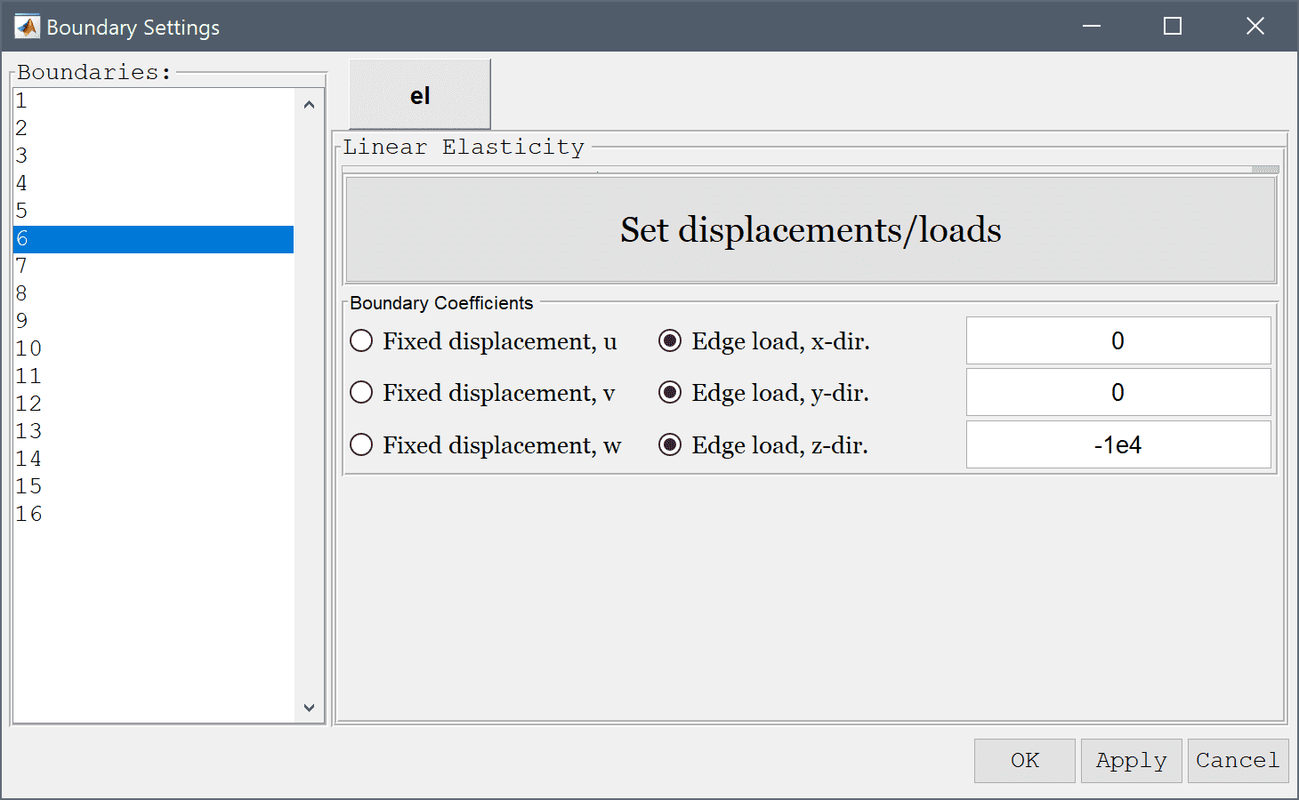
Lastly select the far right boundary (here boundary number 6) and select set an Edge load in the z-direction with the value -1e4. Press OK to finish prescribing boundary conditions.
Now that the problem is fully specified, press the Solve Mode Toolbar button to switch to solve mode. Then press the = Tool button to call the solver with the default solver settings.

After the problem has been solved FEATool will automatically switch to postprocessing mode and here display the computed von Mieses stress. To change the plot, open the postprocessing settings dialog box by clicking on the Plot Options Toolbar button and select z-displacement from the pre-defined Surface Plot expressions. The deformation plot can also be used to see how the model will deform under load.

Press the Plot Options Toolbar button.
Select z-displacement from the Predefined surface plot expressions drop-down menu.
Select the Deformation Plot check box.
Select Displacement field from the Predefined deformation plot expressions drop-down menu.
Enter 0.3 into the Deformation scale factor edit field.
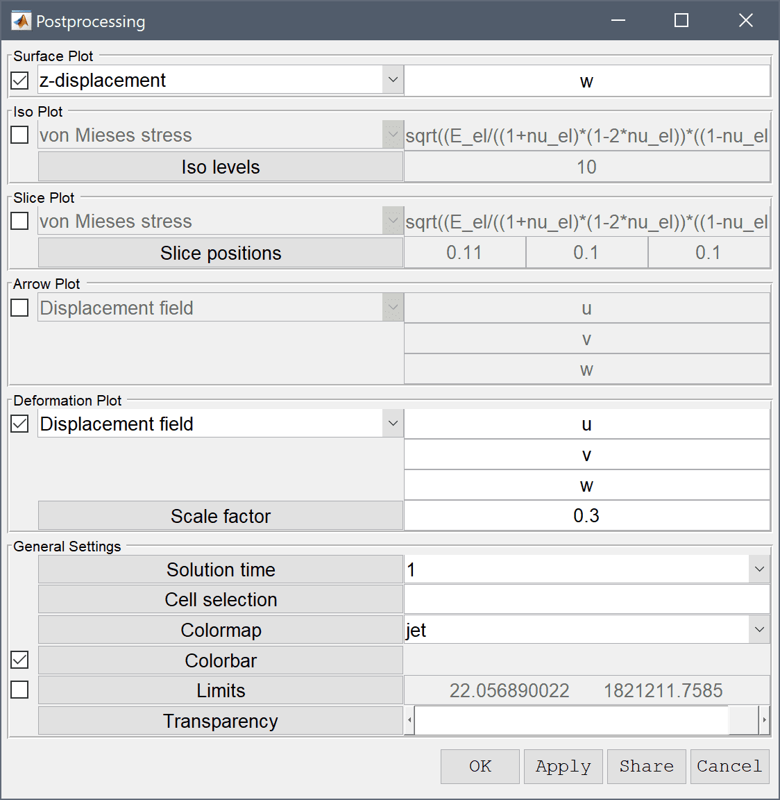
Press OK to plot and visualize the selected postprocessing options.

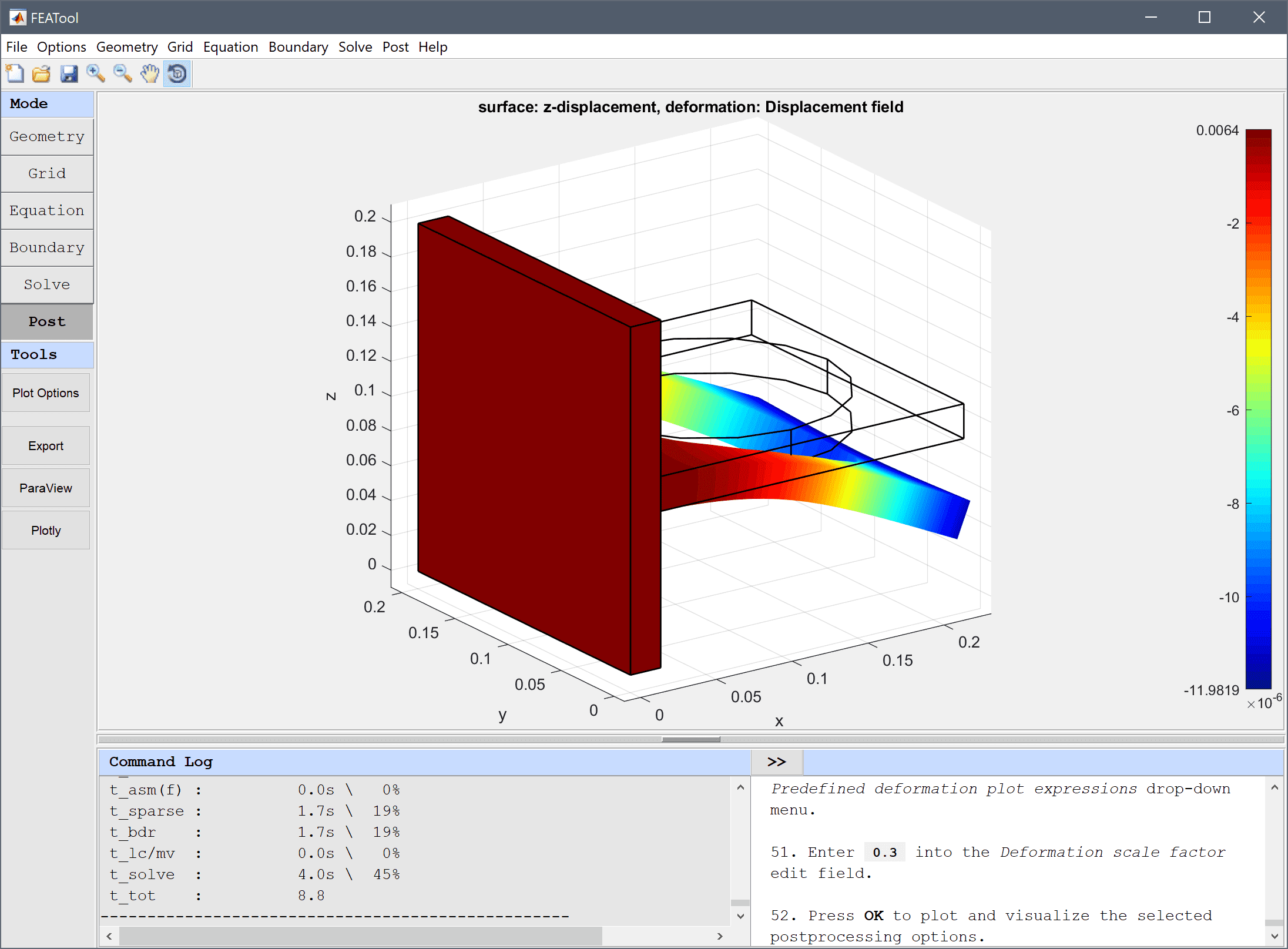
One can see that the maximum displacement occurs at the outer edge and has a magnitude of about 1.2·10^-5 m in the negative z-direction as is to be expected.

The deflection of a bracket structural mechanics model has now been completed and can be saved as a binary (.fea) model file, or exported as a programmable MATLAB m-script text file, or GUI script (.fes) file.

Parametric Study

Parametric studies can be very useful tools to clearly see how a model will behave under varying conditions. The following section presents a parametric study of the bracket model varying both the geometry, in this case plate thickness, and also the applied load force.

The first step in creating a parametric model is to save the model as an m-script model file. This can be done by selecting Save as MATLAB Script... from the File menu.
Open the file in your favorite editor. It is now possible to see exactly which steps and functions were used in creating the model. The first change to make is to add vectors of parameters at the top of the file
```
 thickness = [ 0.02 0.015 0.01 0.008 ];
 loads     = [ 1e4 2e4 1e5 1e6 ];
```

The second change is to replace the geometry and grid operations with the following code so that the thickness of the second block will be varied with the iteration counter i

 for i=1:length(thickness)

 % Geometry operations.
 fea.geom = struct;
 gobj = gobj_block( 0, 0.02, 0, 0.2, 0, 0.2, 'B1' );
 fea  = geom_add_gobj( fea, gobj );
 gobj = gobj_block( 0, 0.2, 0, 0.2, ...
               0.1-thickness(i)/2, 0.1+thickness(i)/2, 'B1' );
 fea  = geom_add_gobj( fea, gobj );
 gobj = gobj_cylinder( [ 0.1, 0.1, 0.08 ], 0.08, 0.04,3,'C1');
 fea  = geom_add_gobj( fea, gobj );
 fea  = geom_apply_formula( fea, 'B1+B2-C1' );

 % Grid generation.
 fea.grid = gridgen( fea, 'hmax', thickness(i)/2 );

As second loop can now be introduced where the varying load is extracted and prescribed by using a constant variable. The equation settings can be kept from the saved model.
```
 for j=1:length(loads)

 % Constants and expressions.
 fea.expr = { 'load', loads(j) };

 % Equation settings.
 fea.phys.el.dvar = { 'u', 'v', 'w' };
 fea.phys.el.sfun = { 'sflag1', 'sflag1', 'sflag1' };
 fea.phys.el.eqn.coef = { 'nu_el', ', '', { '0.3' };
 ...
```
Two loops have now been set up around the model, the first creating a geometry with varying thickness, and the second will prescribe the varying load. Note that setting up the loops in this way allows reusing the grid in the inner loop and saving computational time.

When the grid changes the boundary numbering may also change. The static boundary condition prescription must therefore be replaced with one that identifies the correct boundaries. This can be achieved in the following way

 % Boundary conditions.
 n_bdr = max(fea.grid.b(3,:));
 ind_fixed = findbdr( fea, 'x<0.005' );
 ind_load  = findbdr( fea, 'x>0.19'  );
 fea.phys.el.bdr.sel = ones(1,n_bdr);

 % Define Homogeneous Neumann BC type.
 n_bdr  = max(fea.grid.b(3,:));
 bctype = num2cell( zeros(3,n_bdr) );

 % Set Dirichlet BCs for the fixed boundary.
 [bctype{:,ind_fixed}] = deal( 1 );
 fea.phys.el.bdr.coef{1,end-2} = bctype;

 % Define all zero BC coefficients.
 bccoef = num2cell( zeros(3,n_bdr) );

 % Apply negative z-load to outer edge.
 [bccoef{3,ind_load}] = deal( '-load' );

 % Store BC coefficient array.
 fea.phys.el.bdr.coef{1,end} = bccoef;

When the problem is fully specified we can call the solver, apply postprocessing to calculate the maximum stress, and close the loops

% Solver call.
fea = parsephys( fea );
fea = parseprob( fea );
fea.sol.u = solvestat( fea );

% Postprocessing.
s_vm = fea.phys.el.eqn.vars{1,2};
vm_stress = evalexpr( s_vm, fea.grid.p, fea );
max_vm_stress(i,j) = max(vm_stress);

end,end

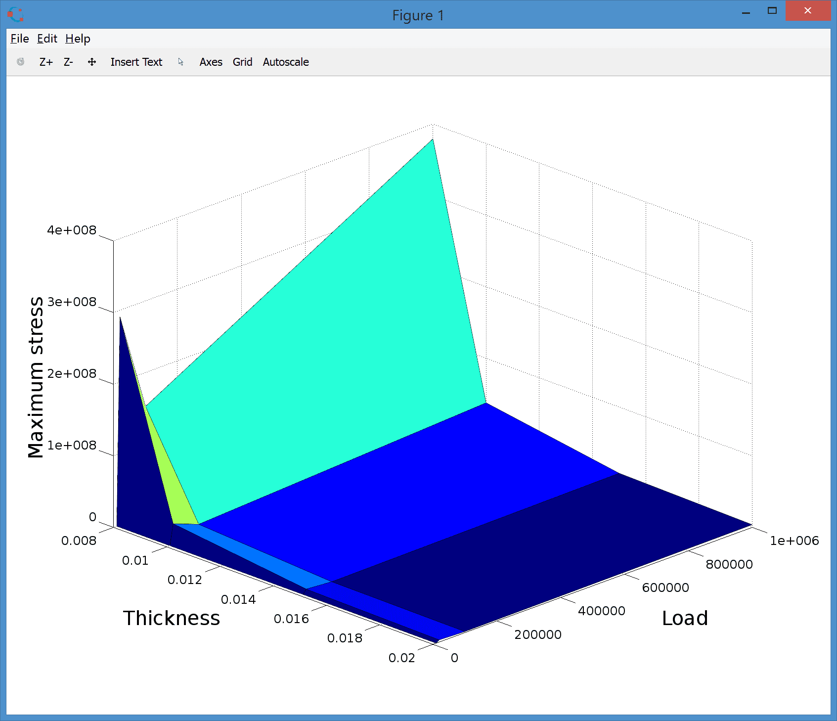
Finally visualize the all computed maximum stresses at once as

% Visualization.
[t,l] = meshgrid(thickness,loads);
surf( t, l, max_vm_stress, log(max_vm_stress) )
xlabel( 'Thickness' )
ylabel( 'Load' )
zlabel( 'Maximum stress' )
view( 45, 30 )

The complete parameter study model can be found as the ex_linearelasticity3 script file in the examples subdirectory of the FEATool installation folder.